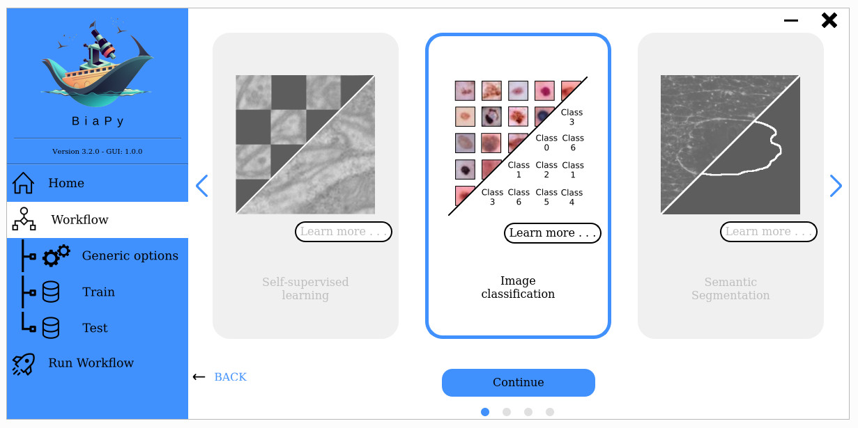
Classification

The goal of this workflow is to assing a label to the input image.

• Input:

  • Image.

• Output:

  • .csv file with the assigned class to each image.

In the figure below a few examples of this workflow’s input are depicted:

Each of these examples are of a different class and were obtained from MedMNIST v2 ([YSW+21]), concretely from DermaMNIST dataset which is a large collection of multi-source dermatoscopic images of common pigmented skin lesions.

Data preparation

Each image label is obtained from the directory name in which that image resides. That is why is so important to follow the directory tree as described below. If you have a .csv file with each image label, as is provided by MedMNIST v2, you can use our script from_class_csv_to_folders.py to create the directory tree as below:

dataset/
├── train
│   ├── 0
│   │   ├── train0_0.png
│   │   ├── train1013_0.png
│   │   ├── . . .
│   │   └── train932_0.png
│   ├── 1
│   │   ├── train104_1.png
│   │   ├── train1049_1.png
│   │   ├── . . .
│   │   └── train964_1.png
| . . .
│   └── 6
│       ├── train1105_6.png
│       ├── train1148_6.png
│       ├── . . .
│       └── train98_6.png
└── test
    ├── 0
    │   ├── test1008_0.png
    │   ├── test1084_0.png
    │   ├── . . .
    │   └── test914_0.png
    ├── 1
    │   ├── test10_1.png
    │   ├── test1034_1.png
    │   ├── . . .
    │   └── test984_1.png
  . . .
    └── 6
        ├── test1021_6.png
        ├── test1069_6.png
        ├── . . .
        └── test806_6.png

Here each directory is a number but it can be any string. Notice that they will be considered the class names. Regarding the test, if you have no classes it doesn’t matter if the images are separated in several folders or are all in one folder. But, if DATA.TEST.LOAD_GT is enabled, each folder in test path (i.e. DATA.TEST.PATH) will be considered as a class (as done for training and validation).

Configuration file

Find in templates/classification folder of BiaPy a few YAML configuration templates for this workflow.

Special workflow configuration

Here some special configuration options that can be selected in this workflow are described:

• Metrics: during the inference phase the performance of the test data is measured using different metrics if test masks were provided (i.e. ground truth) and, consequently, DATA.TEST.LOAD_GT is enabled. In the case of classification the accuracy, precision, recall, and F1 are calculated. Apart from that, the confusion matrix is also printed.

Run

Command lineDockerGoogle Colab

Open a terminal as described in Installation. For instance, using 2d_classification.yaml template file, the code can be run as follows:

# Configuration file
job_cfg_file=/home/user/2d_classification.yaml
# Where the experiment output directory should be created
result_dir=/home/user/exp_results
# Just a name for the job
job_name=my_2d_classification
# Number that should be increased when one need to run the same job multiple times (reproducibility)
job_counter=1
# Number of the GPU to run the job in (according to 'nvidia-smi' command)
gpu_number=0

# Move where BiaPy installation resides
cd BiaPy

# Load the environment
conda activate BiaPy_env
source $CONDA_PREFIX/etc/conda/activate.d/env_vars.sh

python -u main.py \
    --config $job_cfg_file \
    --result_dir $result_dir  \
    --name $job_name    \
    --run_id $job_counter  \
    --gpu $gpu_number

For multi-GPU training you can call BiaPy as follows:

gpu_number="0, 1, 2"
python -u -m torch.distributed.run \
    --nproc_per_node=3 \
    main.py \
    --config $job_cfg_file \
    --result_dir $result_dir  \
    --name $job_name    \
    --run_id $job_counter  \
    --gpu $gpu_number

nproc_per_node need to be equal to the number of GPUs you are using (e.g. gpu_number length).

Results

The main output of this workflow will be a file named predictions.csv that will contain the predicted image class:

Classification workflow output

All files are placed in results folder under --result_dir directory with the --name given. Following the example, you should see that the directory /home/user/exp_results/classification has been created. If the same experiment is run 5 times, varying --run_id argument only, you should find the following directory tree:

my_2d_classification/
├── config_files/
│   └── 2d_classification.yaml
├── checkpoints
│   └── model_weights_classification_1.h5
└── results
    ├── my_2d_classification_1
    ├── . . .
    └── my_2d_classification_5
        ├── predictions.csv
        ├── aug
        │   └── .tif files
        ├── charts
        │   ├── my_2d_classification_1_*.png
        │   ├── my_2d_classification_1_loss.png
        │   └── model_plot_my_2d_classification_1.png
        ├── train_logs
        └── tensorboard

• config_files: directory where the .yaml filed used in the experiment is stored.

  • 2d_classification.yaml: YAML configuration file used (it will be overwrited every time the code is run).

• checkpoints: directory where model’s weights are stored.

  • model_weights_my_2d_classification_1.h5: checkpoint file (best in validation) where the model’s weights are stored among other information.

  • normalization_mean_value.npy: normalization mean value (only created if DATA.NORMALIZATION.TYPE is custom). Is saved to not calculate it everytime and to use it in inference.

  • normalization_std_value.npy: normalization std value (only created if DATA.NORMALIZATION.TYPE is custom). Is saved to not calculate it everytime and to use it in inference.

• results: directory where all the generated checks and results will be stored. There, one folder per each run are going to be placed.

  • my_2d_classification_1: run 1 experiment folder.

    • predictions.csv: list of assigned class per test image.

    • aug: image augmentation samples.

    • charts:

      • my_2d_classification_1_*.png: Plot of each metric used during training.

      • my_2d_classification_1_loss.png: Loss over epochs plot (when training is done).

      • model_plot_my_2d_classification_1.png: plot of the model.

• train_logs: each row represents a summary of each epoch stats. Only avaialable if training was done.

• tensorboard: Tensorboard logs.

Note

Here, for visualization purposes, only my_2d_classification_1 has been described but my_2d_classification_2, my_2d_classification_3, my_2d_classification_4 and my_2d_classification_5 directories will follow the same structure.