Detection
The goal of this workflow is to localize objects in the input image, not requiring a pixel-level class. Common strategies produce either bounding boxes containing the objects or individual points at their center of mass [ZWKrahenbuhl19], which is the one adopted by BiaPy.
Input:
Image (single-channel or multi-channel). E.g. image with shape
(500, 500, 1)(y, x, channels)in2Dor(100, 500, 500, 1)(z, y, x, channels)in3D..csvfile containing the list of points to detect.
Output:
Image with the detected points as white dots.
.csvfile with the list of detected points in napari format.A
_prob.csvfile with the same list of points as above but now with their detection probability (also in napary format).
In the figure below an example of this workflow’s input is depicted:
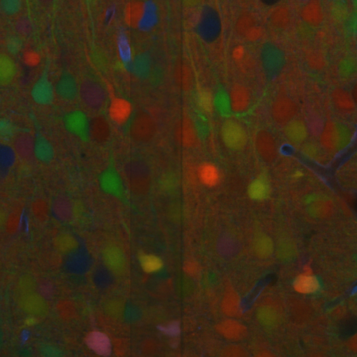
Input image. |
Input |
Description of the .csv file:
Each row represents the middle point of the object to be detected. Each column is a coordinate in the image dimension space.
The first column name does not matter but it needs to be there. No matter also the enumeration and order for that column.
If the images are
3D, three columns need to be present and their names must be[axis-0, axis-1, axis-2], which represent(z,y,x)axes. If the images are2D, only two columns are required[axis-0, axis-1], which represent(y,x)axes.For multi-class detection problem, i.e.
MODEL.N_CLASSES > 1, add an additionalclasscolumn to the file. The classes need to start from1and consecutive, i.e.1,2,3,4...and not like1,4,8,6....Coordinates can be float or int but they will be converted into ints so they can be translated to pixels.
Data preparation
To ensure the proper operation of the library the data directory tree should be something like this:
Warning
In this workflow the name of each .tif file and its corresponding .csv file must be the same.
Problem resolution
Firstly, a pre-processing step is done where the list of points of the .csv file is transformed into point mask images. During this process some checks are made to ensure there is not repeated point in the .csv. This option is True by default with PROBLEM.DETECTION.CHECK_POINTS_CREATED so if any problem is found the point mask of that .csv will not be created until the problem is solve.
After the train phase, the model output will be an image where each pixel of each channel will have the probability (in [0-1] range) of being of the class that represents that channel. The image would be something similar to the left picture below:

Model output. |
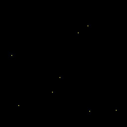
Final points considered. |
So those probability images, as the left picture above, can be converted into the final points, as the rigth picture above, we use peak_local_max function to find peaks in those probability clouds. For that, you need to define a threshold, TEST.DET_MIN_TH_TO_BE_PEAK variable in our case, for the minimum probability to be considered as a point. You can set different thresholds for each class in TEST.DET_MIN_TH_TO_BE_PEAK, e.g. [0.7,0.9].
Configuration file
Find in templates/detection folder of BiaPy a few YAML configuration templates for this workflow.
Special workflow configuration
Metrics
During the inference phase the performance of the test data is measured using different metrics if test masks were provided (i.e. ground truth) and, consequently, DATA.TEST.LOAD_GT is True. In the case of detection, the Intersection over Union (IoU) is measured after network prediction:
IoU metric, also referred as the Jaccard index, is essentially a method to quantify the percent of overlap between the target mask and the prediction output. Depending on the configuration different values are calculated (as explained in Test phase and Metric measurement). This values can vary a lot as stated in [FBMunozBAC21].
Per patch: IoU is calculated for each patch separately and then averaged.
Reconstructed image: IoU is calculated for each reconstructed image separately and then averaged. Notice that depending on the amount of overlap/padding selected the merged image can be different than just concatenating each patch.
Full image: IoU is calculated for each image separately and then averaged. The results may be slightly different from the reconstructed image.
Then, after extracting the final points from the predictions, precision, recall and F1 are defined as follows:
Precision, is the fraction of relevant points among the retrieved points. More info here.
Recall, is the fraction of relevant points that were retrieved. More info here.
F1, is the harmonic mean of the precision and recall. More info here.
The last three metrics, i.e. precision, recall and F1, use TEST.DET_TOLERANCE to determine when a point is considered as a true positive. In this process the test resolution is also taken into account. You can set different tolerances for each class, e.g. [10,15].
Post-processing
After network prediction and applied to 3D images (e.g. PROBLEM.NDIM is 2D or TEST.ANALIZE_2D_IMGS_AS_3D_STACK is True). There are the following options:
Z-filtering: to apply a median filtering in
zaxis. Useful to maintain class coherence across3Dvolumes. Enable it withTEST.POST_PROCESSING.Z_FILTERINGand useTEST.POST_PROCESSING.Z_FILTERING_SIZEfor the size of the median filter.YZ-filtering: to apply a median filtering in
yandzaxes. Useful to maintain class coherence across3Dvolumes that can work slightly better thanZ-filtering. Enable it withTEST.POST_PROCESSING.YZ_FILTERINGand useTEST.POST_PROCESSING.YZ_FILTERING_SIZEfor the size of the median filter.
Then, after extracting the final points from the predictions, the following post-processing methods are avaialable:
Remove close points: to remove redundant close points to each other within a certain radius (controlled by
TEST.POST_PROCESSING.REMOVE_CLOSE_POINTS). The radius value can be specified using the variableTEST.POST_PROCESSING.REMOVE_CLOSE_POINTS_RADIUS. You can set different radius for each class, e.g.[0.7,0.9]. In this post-processing is important to setDATA.TEST.RESOLUTION, specially for3Ddata where the resolution inzdimension is usually less than in other axes. That resolution will be taken into account when removing points.Create instances from points: Once the points have been detected and any close points have been removed, it is possible to create instances from the remaining points. The variable
TEST.POST_PROCESSING.DET_WATERSHEDcan be set to perform this step. However, sometimes cells have low contrast in their centers, for example due to the presence of a nucleus. This can result in the seed growing to fill only the nucleus while the cell is much larger. In order to address the issue of limited growth of certain types of seeds, a process has been implemented to expand the seeds beyond the borders of their nuclei. This process allows for improved growth of these seeds. To ensure that this process is applied only to the appropriate cells, variables such asTEST.POST_PROCESSING.DET_WATERSHED_DONUTS_CLASSES,TEST.POST_PROCESSING.DET_WATERSHED_DONUTS_PATCH, andTEST.POST_PROCESSING.DET_WATERSHED_DONUTS_NUCLEUS_DIAMETERhave been created. It is important to note that these variables are necessary to prevent the expansion of the seed beyond the boundaries of the cell, which could lead to expansion into the background.
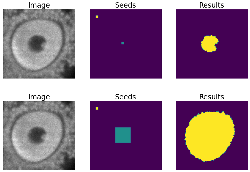
For left to right: raw image, initial seeds for the watershed and the resulting instances after growing the seeds. In the first row the problem with nucleus visible type cells is depicted, where the central seed can not be grown more than the nucleus border. On the second row the solution of dilating the central point is depicted.
Run
Select detection workflow during the creation of a new configuration file:
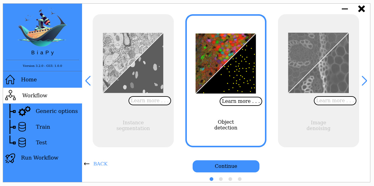
Open a terminal as described in Installation. For instance, using 2d_detection.yaml template file, the code can be run as follows:
# Configuration file
job_cfg_file=/home/user/2d_detection.yaml
# Path to the data directory
data_dir=/home/user/data
# Where the experiment output directory should be created
result_dir=/home/user/exp_results
# Just a name for the job
job_name=my_2d_detection
# Number that should be increased when one need to run the same job multiple times (reproducibility)
job_counter=1
# Number of the GPU to run the job in (according to 'nvidia-smi' command)
gpu_number=0

docker run --rm \
    --gpus "device=$gpu_number" \
    --mount type=bind,source=$job_cfg_file,target=$job_cfg_file \
    --mount type=bind,source=$result_dir,target=$result_dir \
    --mount type=bind,source=$data_dir,target=$data_dir \
    BiaPyX/biapy \
        -cfg $job_cfg_file \
        -rdir $result_dir \
        -name $job_name \
        -rid $job_counter \
        -gpu $gpu_number
Note
Note that data_dir must contain all the paths DATA.*.PATH and DATA.*.GT_PATH so the container can find them. For instance, if you want to only train in this example DATA.TRAIN.PATH and DATA.TRAIN.GT_PATH could be /home/user/data/train/x and /home/user/data/train/y respectively.
Open a terminal as described in Installation. For instance, using 2d_detection.yaml template file, the code can be run as follows:
# Configuration file
job_cfg_file=/home/user/2d_detection.yaml
# Where the experiment output directory should be created
result_dir=/home/user/exp_results
# Just a name for the job
job_name=my_2d_detection
# Number that should be increased when one need to run the same job multiple times (reproducibility)
job_counter=1
# Number of the GPU to run the job in (according to 'nvidia-smi' command)
gpu_number=0

# Move where BiaPy installation resides
cd BiaPy

# Load the environment
conda activate BiaPy_env

python -u main.py \
    --config $job_cfg_file \
    --result_dir $result_dir  \
    --name $job_name    \
    --run_id $job_counter  \
    --gpu $gpu_number
For multi-GPU training you can call BiaPy as follows:
gpu_number="0, 1, 2"
python -u -m torch.distributed.run \
    --nproc_per_node=3 \
    main.py \
    --config $job_cfg_file \
    --result_dir $result_dir  \
    --name $job_name    \
    --run_id $job_counter  \
    --gpu $gpu_number
nproc_per_node need to be equal to the number of GPUs you are using (e.g. gpu_number length).
Results
The results are placed in results folder under --result_dir directory with the --name given.
Following the example, you should see that the directory /home/user/exp_results/my_2d_detection has been created. If the same experiment is run 5 times, varying --run_id argument only, you should find the following directory tree:
config_files: directory where the .yaml filed used in the experiment is stored.my_2d_detection.yaml: YAML configuration file used (it will be overwrited every time the code is run).
checkpoints: directory where model’s weights are stored.my_2d_detection_1-checkpoint-best.pth: checkpoint file (best in validation) where the model’s weights are stored among other information.normalization_mean_value.npy: normalization mean value (only created ifDATA.NORMALIZATION.TYPEiscustom). Is saved to not calculate it everytime and to use it in inference.normalization_std_value.npy: normalization std value (only created ifDATA.NORMALIZATION.TYPEiscustom). Is saved to not calculate it everytime and to use it in inference.
results: directory where all the generated checks and results will be stored. There, one folder per each run are going to be placed.my_2d_detection_1: run 1 experiment folder.cell_counter.csv: file with a counter of detected objects for each test sample.aug: image augmentation samples.charts:my_2d_detection_1_*.png: Plot of each metric used during training.my_2d_detection_1_loss.png: Loss over epochs plot (when training is done).model_plot_my_2d_detection_1.png: plot of the model.
per_image:.tif files: reconstructed images from patches.
full_image(optional ifTEST.FULL_IMGisTrue):.tif files: full image predictions.
per_image_local_max_check:.tif files: Same asper_imagebut with the final detected points.
point_associations: optional. Only if ground truth was provided..tif files: prediction (_pred_ids) and ground truth (_gt_ids) ids..csv files: false positives (_fp) and ground truth associations (_gt_assoc).
train_logs: each row represents a summary of each epoch stats. Only avaialable if training was done.tensorboard: Tensorboard logs.
Note
Here, for visualization purposes, only my_2d_detection_1 has been described but my_2d_detection_2, my_2d_detection_3, my_2d_detection_4 and my_2d_detection_5 will follow the same structure.