Instance segmentation

Description of the task

The goal of this workflow is assign a unique ID, i.e. an integer value, to each object of the input image, thus producing a label image with instance masks. An example of this task is displayed in the figure below, with an electron microscopy image used as input (left) and its corresponding instance label image identifying each invididual mitochondrion (rigth). Each color in the mask image corresponds to a unique object.

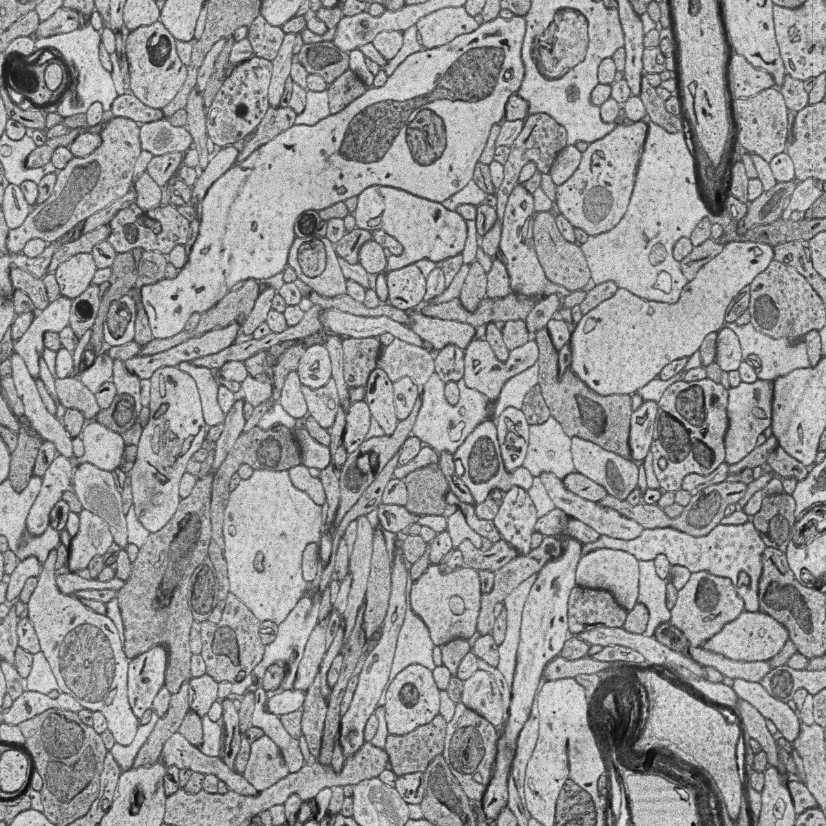
Input image (electron microscopy, from the MitoEM dataset).

Label image with mitochondria instance masks.

Each instance may also contain information about its class (optional). In that case, the label image will contain two channels, one with the instance IDs and one with their corresponding semantic (class) labels. An example of this setting is depicted below:

Instance and classification setting example. From right to left: input raw image (histology image from CoNIC Challenge) and its corresponding label image with instance masks (channel 0) and classification/semantic masks (channel 1).

Inputs and outputs

The instance segmentation workflows in BiaPy expect a series of folders as input:

• Training Raw Images: A folder that contains the unprocessed (single-channel or multi-channel) images that will be used to train the model.

  Expand to see how to configure

  GUIGoogle Colab / NotebooksYAML configuration file

  In the current BiaPy GUI, this option is defined through the Wizard questions. Alternatively, you can edit the DATA.TRAIN.PATH in your YAML file before clicking Run Workflow and loading that YAML file.

• Training Label Images: A folder that contains the instance label (single- or multi-channel) images for training. Ensure the number and dimensions match the training raw images.

  Expand to see how to configure

  GUIGoogle Colab / NotebooksYAML configuration file

  In the current BiaPy GUI, this option is defined through the Wizard questions. Alternatively, you can edit the DATA.TRAIN.GT_PATH in your YAML file before clicking Run Workflow and loading that YAML file.

  Note

  Remember the label images need to be single-channel when performing instance segmentation only, and multi-channel in the instance and classification setting (first channel for instance labels and second channel for semantic labels).

• [Optional] Test Raw Images: A folder that contains the images to evaluate the model's performance.
  Expand to see how to configure

  GUIGoogle Colab / NotebooksYAML configuration file

  In the current BiaPy GUI, this option is defined through the Wizard questions. Alternatively, you can edit the DATA.TEST.PATH in your YAML file before clicking Run Workflow and loading that YAML file.

• [Optional] Test Label Images: A folder that contains the instance label images for testing. Again, ensure their count and sizes align with the test raw images.
  Expand to see how to configure

  GUIGoogle Colab / NotebooksYAML configuration file

  In the current BiaPy GUI, this option is defined through the Wizard questions. Alternatively, you can edit the DATA.TEST.GT_PATH in your YAML file before clicking Run Workflow and loading that YAML file.

  Note

  Remember the label images need to be single-channel when performing instance segmentation only, and multi-channel in the instance and classification setting (first channel for instance labels and second channel for semantic labels).

Upon successful execution, a directory will be generated with the segmentation results. Therefore, you will need to define:

• Output Folder: A designated path to save the segmentation outcomes.

  Expand to see how to configure

  GUIGoogle Colab / NotebooksCommand line

  Under Run Workflow, click on the Browse button of Output folder to save the results:

  

BiaPy input and output folders for instance segmentation.

Data structure

To ensure the proper operation of the library, the data directory tree should be something like this:

dataset/
├── train
│   ├── raw
│   │   ├── training-0001.tif
│   │   ├── training-0002.tif
│   │   ├── . . .
│   │   └── training-9999.tif
│   └── label
│       ├── training_groundtruth-0001.tif
│       ├── training_groundtruth-0002.tif
│       ├── . . .
│       └── training_groundtruth-9999.tif
└── test
    ├── raw
    │   ├── testing-0001.tif
    │   ├── testing-0002.tif
    │   ├── . . .
    │   └── testing-9999.tif
    └── label
        ├── testing_groundtruth-0001.tif
        ├── testing_groundtruth-0002.tif
        ├── . . .
        └── testing_groundtruth-9999.tif

In this example, the raw training images are under dataset/train/raw/ and their corresponding labels are under dataset/train/label/, while the raw test images are under dataset/test/raw/ and their corresponding labels are under dataset/test/label/. This is just an example, you can name your folders as you wish as long as you set the paths correctly later.

Note

Ensure that images and their corresponding masks are sorted in the same way. A common approach is to fill with zeros the image number added to the filenames (as in the example).

Example datasets

Below is a list of publicly available datasets that are ready to be used in BiaPy for instance segmentation:

Example dataset	Image dimensions	Link to data
StarDist V2	2D	Stardist_v2.zip
3D demo (from StarDist 0.3.0 release)	3D	demo3D.zip
CartoCell dataset	3D	CartoCell.zip

Minimal configuration

Apart from the input and output folders, there are a few basic parameters that always need to be specified in order to run an instance segmentation workflow in BiaPy. Depending on the parameter, they can be defined through the GUI Wizard, in the code-free notebooks, or by editing the YAML configuration file.

Experiment name

Also known as “model name” or “job name”, this will be the name of the current experiment you want to run, so it can be differenciated from other past and future experiments.

Expand to see how to configure

GUIGoogle Colab / NotebooksCommand line

Under Run Workflow, type the name you want for the job in the Job name field:

Note

Use only my_model -style, not my-model (Use “_” not “-“). Do not use spaces in the name. Avoid using the name of an existing experiment/model/job (saved in the same result folder) as it will be overwritten.

Data management

Validation Set

With the goal to monitor the training process, it is common to use a third dataset called the “Validation Set”. This is a subset of the whole dataset that is used to evaluate the model’s performance and optimize training parameters. This subset will not be directly used for training the model, and thus, when applying the model to these images, we can see if the model is learning the training set’s patterns too specifically or if it is generalizing properly.

Graphical description of data partitions in BiaPy.

To define such set, there are two options:

• Validation proportion/percentage: Select a proportion (or percentage) of your training dataset to be used to validate the network during the training. Usual values are 0.1 (10%) or 0.2 (20%), and the samples of that set will be selected at random.

  Expand to see how to configure

  GUIGoogle Colab / NotebooksYAML configuration file

  In the current BiaPy GUI, this option is configured by editing the DATA.VAL.SPLIT_TRAIN in your YAML file before clicking Run Workflow and loading that YAML file.

• Validation paths: Similar to the training and test sets, you can select two folders with the validation raw and label images:

  • Validation Raw Images: A folder that contains the unprocessed (single-channel or multi-channel) images that will be used to select the best model during training.

    Expand to see how to configure

    GUIGoogle Colab / NotebooksYAML configuration file

    In the current BiaPy GUI, this option is configured by editing the DATA.VAL.PATH in your YAML file before clicking Run Workflow and loading that YAML file.

  • Validation Label Images: A folder that contains the instance label (single-channel) images for validation. Ensure the number and dimensions match those of the validation raw images.

    Expand to see how to configure

    GUIGoogle Colab / NotebooksYAML configuration file

    In the current BiaPy GUI, this option is configured by editing the DATA.VAL.GT_PATH in your YAML file before clicking Run Workflow and loading that YAML file.

    Note

    Remember the label images need to be single-channel when performing instance segmentation only, and multi-channel in the instance and classification setting (first channel for instance labels and second channel for semantic labels).

Test ground-truth

Do you have labels for the test set? This is a key question so BiaPy knows if your test set will be used for evaluation in new data (unseen during training) or simply produce predictions on that new data. All workflows contain a parameter to specify this aspect.

Expand to see how to configure

GUIGoogle Colab / NotebooksYAML configuration file

In the current BiaPy GUI, this option is defined through the Wizard questions. Alternatively, you can edit the DATA.TEST.LOAD_GT in your YAML file before clicking Run Workflow and loading that YAML file.

Basic training parameters

At the core of each BiaPy workflow there is a deep learning model. Although we try to simplify the number of parameters to tune, these are the basic parameters that need to be defined for training an instance segmentation workflow:

• Number of input channels: The number of channels of your raw images (grayscale = 1, RGB = 3). Notice the dimensionality of your images (2D/3D) is set by default depending on the workflow template you select.

  Expand to see how to configure

  GUIGoogle Colab / NotebooksYAML configuration file

  In the current BiaPy GUI, this option is configured by editing the DATA.PATCH_SIZE in your YAML file before clicking Run Workflow and loading that YAML file.

• Number of epochs: This number indicates how many rounds the network will be trained. On each round, the network usually sees the full training set. The value of this parameter depends on the size and complexity of each dataset. You can start with something like 100 epochs and tune it depending on how fast the loss (error) is reduced.

  Expand to see how to configure

  GUIGoogle Colab / NotebooksYAML configuration file

  In the current BiaPy GUI, this option is configured by editing the TRAIN.EPOCHS in your YAML file before clicking Run Workflow and loading that YAML file.

• Patience: This is a number that indicates how many epochs you want to wait without the model improving its results in the validation set to stop training. Again, this value depends on the data you’re working on, but you can start with something like 20.

  Expand to see how to configure

  GUIGoogle Colab / NotebooksYAML configuration file

  In the current BiaPy GUI, this option is configured by editing the TRAIN.PATIENCE in your YAML file before clicking Run Workflow and loading that YAML file.

For improving performance, other advanced parameters can be optimized, for example, the model’s architecture. The architecture assigned as default is the U-Net, as it is effective in instance segmentation tasks. This architecture allows a strong baseline, but further exploration could potentially lead to better results.

Note

Once the parameters are correctly assigned, the training phase can be executed. Note that to train large models effectively the use of a GPU (Graphics Processing Unit) is essential. This hardware accelerator performs parallel computations and has larger RAM memory compared to the CPUs, which enables faster training times.

How to run

BiaPy offers different options to run workflows depending on your degree of computer expertise. Select whichever is more approppriate for you:

GUIGoogle ColabDockerCommand line

In the BiaPy GUI, click on the Wizard, then follow the next instructions to select the instance segmentation workflow:

Step 1: Choose a folder and file name to store your workflow configuration file, then click "Start".

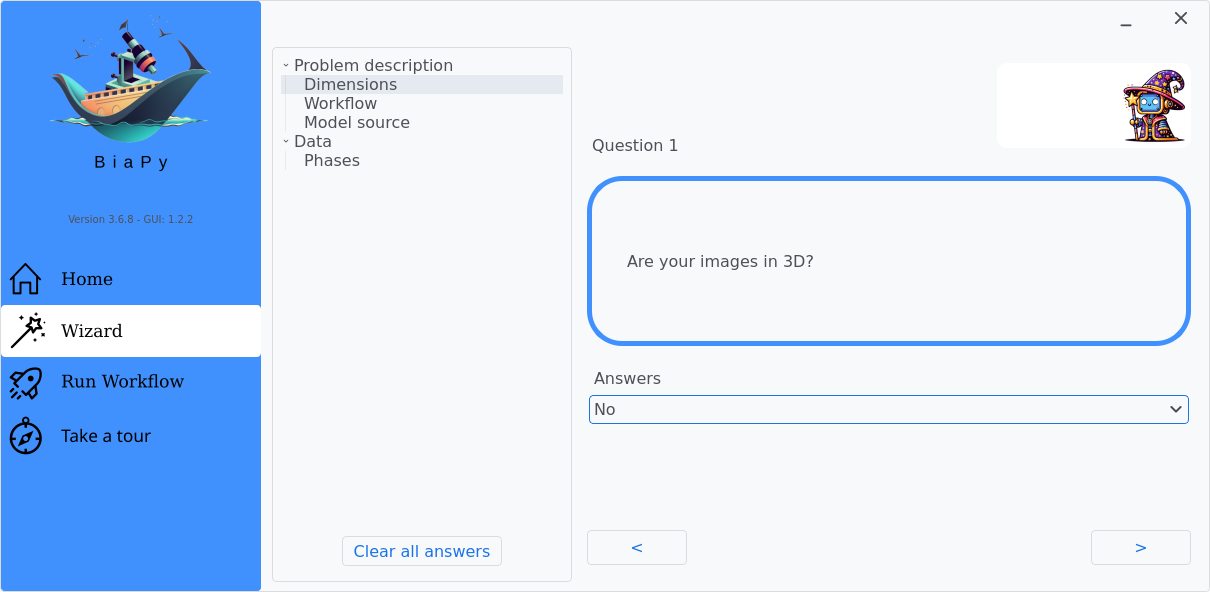
Step 2: Under Question 1, select the answer that best fits with your data dimensionality.

Step 3: Under Question 2, select the answer "Generate masks of different objects/regions within the image".

Previous Next

After that, you will be able to edit the parameters of the workflow and run it.

Note

BiaPy’s GUI requires that all data and configuration files reside on the same machine where the GUI is being executed.

For a full example on how to configure an instance segmentation workflow in BiaPy GUI, watch our instance segmentation demo video:

Tip

If you need additional help, watch BiaPy’s GUI walkthrough video.

Templates

In the templates/instance_segmentation folder of BiaPy, you will find a few YAML configuration templates for this workflow.

[Advanced] Special workflow configuration

Note

This section is recommended for experienced users only to improve the performance of their workflows. When in doubt, do not hesitate to check our FAQ & Troubleshooting or open a question in the image.sc discussion forum.

Advanced parameters

Many of the parameters of our workflows are set by default to values that work commonly well. However, it may be needed to tune them to improve the results of the workflow. For instance, you may modify the following parameters

• Model architecture: Select the architecture of the deep neural network used as backbone of the pipeline. Options: U-Net, Residual U-Net, Attention U-Net, SEUNet, MultiResUNet, ResUNet++, UNETR-Mini, UNETR-Small, UNETR-Base, ResUNet SE and U-NeXt V1. Default value: U-Net.

• Batch size: This parameter defines the number of patches seen in each training step. Reducing or increasing the batch size may slow or speed up your training, respectively, and can influence network performance. Common values are 4, 8, 16, etc.

• Patch size: Input the size of the patches use to train your model (length in pixels in X and Y). The value should be smaller or equal to the dimensions of the image. The default value is 256 in 2D, i.e. 256x256 pixels.

• Optimizer: Select the optimizer used to train your model. Options: ADAM, ADAMW, Stochastic Gradient Descent (SGD). ADAM usually converges faster, while ADAMW provides a balance between fast convergence and better handling of weight decay regularization. SGD is known for better generalization. Default value: ADAMW.

• Initial learning rate: Input the initial value to be used as learning rate. If you select ADAM as optimizer, this value should be around 10e-4.

• Learning rate scheduler: Select to adjust the learning rate between epochs. The current options are “Reduce on plateau”, “One cycle”, “Warm-up cosine decay” or no scheduler.

• Test time augmentation (TTA): Select to apply augmentation (flips and rotations) at test time. It usually provides more robust results but uses more time to produce each result. By default, no TTA is peformed.

Problem representation

In BiaPy the instance segmentation problem is solved using a bottom-up approach. This means that a preprocessing step transforms the input per-pixel instance labels into a multi-channel representation that the network will learn (and subsequently predict). After that, these representations are fused to produce the final instance segmentation. In BiaPy we have integrated many different representations that can configured via the PROBLEM.INSTANCE_SEG.DATA_CHANNELS variable. An possible representation is depicted in the following figure:

Process of F + C + Db representation. From instance
segmentation labels (left) to foreground (F), contour (C) and distance to boundary (Db) masks (right).

---

Channels

Each channel type encodes a different geometric or semantic property of the instances. You select which ones to generate with PROBLEM.INSTANCE_SEG.DATA_CHANNELS (see below). Apart from that, each channel have its own configuration options (e.g. contour thickness, distance transform type, etc.) under PROBLEM.INSTANCE_SEG.DATA_CHANNELS_EXTRA_OPTS.

The currently supported instance channels are:

• Foreground mask (F): Binary mask of all instance interiors (previously called B). Pixels inside any instance (excluding the explicit contour channel) are 1, background is 0. This is usually the main semantic channel for the instances. The extra options for this channel are the following:

  • erosion: Number of pixels to erode the foreground mask. This can help to separate touching instances by removing thin connections. Default is 0 (no erosion).

  • dilation: Number of pixels to dilate the foreground mask. This can help to include uncertain boundary regions into the foreground. Default is 0 (no dilation).

• Background mask (B): Binary mask of all background pixels. Pixels outside any instance are 1, instance interiors are 0. This channel can be useful to explicitly model the background class. The extra options for this channel are the following:

  • erosion: Number of pixels to erode the background mask. This can help to exclude uncertain boundary regions from the background. Default is 0 (no erosion).

  • dilation: Number of pixels to dilate the background mask. This can help to separate touching instances by removing thin connections. Default is 0 (no dilation).

• Center parts (P): Binary mask of center parts of each instance. These centers can be used as seed points for instance separation. The extra options for this channel are the following:

  • type: Type of peak representation. Options are: 'centroid' (single pixel at the instance centroid) and 'skeleton' (skeleton of the instance). Default is 'centroid'.

  • dilation: Number of pixels to dilate the peaks. This can help to create larger seed regions for better instance separation. Default is 1.

  • erosion: Number of pixels to erode the peaks. This can be useful when using skeletons as peaks to make them thinner. Default is 0.

• Contour / boundary (C): Binary mask of object contours. Pixels on the boundary between instance and background (or between touching instances) are 1, the rest are 0. The contour thickness and how it is computed are controlled by the instance channel configuration options. The extra options for this channel are the following:

  • mode: How to compute the contour pixels. Options are: 'thick', 'inner', 'outer', 'subpixel' and 'dense' (as defined in skimage.segmentation.find_boundaries). Default is 'thick'.

• Touching areas (T): Binary mask of pixels that lie in touching regions between two or more instances. This channel is useful to explicitly highlight contact zones that are hard to separate using only F and C. The extra options for this channel are the following:

  • thickness: Thickness in pixels of the touching area. Default is 2.

• Distance to boundary (foreground) (Db): Float mask where each pixel value is the Euclidean distance to the nearest instance boundary, computed inside the instances. Background pixels are typically set to 0 (or a constant). This generalises the old D channel used in previous versions. Intuitively, inside each instance, values increase when moving away from the boundary towards the instance centre. This channel is useful to separate touching instances and to regularise instance shapes. The extra options for this channel are the following:

  • norm: Whether to normalize the distances between 0 and 1. Default is True.

  • mask_values: Whether to mask the distance channel to only calculate the loss in non-zero values. Default is True.

• Distance to center (Dc): Float mask where each pixel value is the Euclidean distance to the instance center/skeleton, computed inside the instances. Background pixels are typically set to 0 (or a constant). This channel can help to better delineate instances from the background and improve separation in crowded regions. The extra options for this channel are the following:

  • type: Type of center representation. Options are: 'centroid' (distance to instance centroid) and 'skeleton' (distance to instance skeleton). Default is 'centroid'.

  • norm: Whether to normalize the distances between 0 and 1. Default is True.

  • mask_values: Whether to mask the distance channel to only calculate the loss in non-zero values. Default is True.

• Distance to boundary (foreground + background) (D): Float mask where the distance-to-boundary information is computed both inside the instances and in the background. Intuitively:

  • inside the instance, values increase when moving away from the boundary towards the instance centre. On the boundary itself, values are 0.

  • in the background, values increase when moving away from the nearest instance.

  This channel is built on top of Db and extends it to the background. It can help to better delineate instances from the background and improve separation in crowded regions. The extra options for this channel are the following:

  • activation: Activation function to be used in the last layer of the model when this channel is selected. Options are: 'tanh' and 'linear'. Default is 'tanh'.

  • alpha: Value to scale the distances of the background when 'act' is 'tanh'. Default is 1.

  • beta: Value to scale the distances of the foreground when 'act' is 'tanh'. Default is 1.

  • norm: Whether to normalize the distances between -1 and 1. Default is True.

• Distance offsets (H, V, Z): Offset (vector field) channels that encode, for each pixel, the displacement towards the instance centre:

  • H – horizontal offset (x-axis).

  • V – vertical offset (y-axis).

  • Z – depth offset (z-axis, only for 3D).

  These channels correspond to Cellpose/Hover-Net/Omnipose-style encodings where instances are recovered from a flow/offset field. The extra options for these channels are the following:

  • norm: Whether to normalize the distances between 0 and 1. Default is True.

  • mask_values: Whether to mask the distance channel to only calculate the loss in non-zero values. Default is True.

• Distance to neighbours (Dn): Float mask encoding how far each pixel is from neighbouring instances. Small values typically occur in crowded regions; larger values appear in isolated instances. This channel can be used to regularise instance shapes and reduce over-segmentation in dense areas. The extra options for this channel are the following:

  • closing_size: Size of the closing to be applied to the combined distance map. Default is 0.

  • norm: Whether to normalize the distances between 0 and 1. Default is True.

  • mask_values: Whether to mask the distance channel to only calculate the loss in non-zero values. Default is True.

  • decline_power: Power to which the distances are raised to control the decline rate. Default is 3.

• Radial distances (R): Radial (star-shaped) distances from each pixel to the instance boundary, in multiple directions (StarDist-like). This channel usually has several internal rays per pixel and is intended for star-convex instance representations. The extra options for this channel are the following:

  • nrays: Number of rays to be used to represent the radial distances. Default is 32 (in 2D) and 96 (in 3D).

  • norm: Whether to normalize the distances between 0 and 1. Default is True.

  • mask_values: Whether to mask the distance channel to only calculate the loss in non-zero values. Default is True.

• Embeddings (E): High-dimensional embedding vectors for each pixel, learned such that pixels belonging to the same instance have similar embeddings, while those from different instances are dissimilar (EmbedSeg-like). This channel is useful for clustering-based instance segmentation approaches and can not be used together with other channels. The extra options for this channel are the following:

  • center_mode: Method to compute the center of the embeddings for each instance during training. Options are 'centroid' (mean embedding) and 'medoid' (most central embedding). Default is 'centroid'.

  • medoid_max_points: Maximum number of points to use when calculating the medoid. Default is 10000.

• Affinities (A): Affinity graphs representing the likelihood of neighboring pixels belonging to the same instance. This channel is useful for dense datasets as in connectomics and can not be used together with other channels. The extra options for this channel are the following:

  • neighborhood: Defines the neighborhood connectivity for the affinity graph. Options are '4-connectivity', '8-connectivity' in 2D, and '6-connectivity', '18-connectivity', '26-connectivity' in 3D. Default is '8-connectivity' in 2D and '26-connectivity' in 3D.

In practice, PROBLEM.INSTANCE_SEG.DATA_CHANNELS is a list (or sequence) of these channel codes (e.g. ['F', 'C', 'Db'] or ['F', 'C', 'H', 'V']). The order of the codes defines the order of the output channels of the network.

For the PROBLEM.INSTANCE_SEG.DATA_CHANNELS_EXTRA_OPTS variable, each channel code can have its own dictionary of extra options (as described above) to further customise how the channel is generated from the instance labels. BiaPy will fill in any missing options with sensible defaults.

---

Channel combinations and weights

• PROBLEM.INSTANCE_SEG.DATA_CHANNELS: List of channel identifiers chosen from F, C, T, Db, D, R, H, V, Z, Dn and E. Examples (non-exhaustive):

  • ['F', 'C'] – classic foreground + contour.

  • ['F', 'C', 'Db'] – foreground + contour + distance to boundary.

  • ['F', 'H', 'V'] – foreground + 2D distance offsets (Cellpose/Hover-Net style).

  • ['Db', 'R'] – foreground + contour + radial distances (StarDist style).

  • ['F', 'C', 'Db', 'Dn'] – foreground + contour + distance to boundary + distance to neighbours.

• PROBLEM.INSTANCE_SEG.DATA_CHANNELS_EXTRA_OPTS: Dictionary of extra options for each channel selected in DATA_CHANNELS. For example, to set the contour to be thick, e.g. 1 pixel inside and 1 pixel outside the true contour, and erode the foreground by 3 pixels, you could set:

  PROBLEM:
    INSTANCE_SEG:
      DATA_CHANNELS: ['F', 'C', 'Db']
      DATA_CHANNELS_EXTRA_OPTS: {'F': {'erosion': 3}, 'C': {'mode': 'thick'}}
  

  See config.py for a full list of channel-specific options.

• PROBLEM.INSTANCE_SEG.DATA_CHANNEL_WEIGHTS: Tuple/list of floats with the same length as DATA_CHANNELS. It sets the relative importance of each channel in the loss. For instance, for DATA_CHANNELS = ['F', 'C', 'Db'] you might set:

  PROBLEM:
    INSTANCE_SEG:
      DATA_CHANNELS: ['F', 'C', 'Db']
      DATA_CHANNEL_WEIGHTS: (1.0, 1.0, 0.5)
  

  so that the distance channel Db has half the impact of the binary channels during training.

During training, the network outputs one prediction map per configured channel. For “binary” channels (F, C, T, etc.), each pixel holds a probability in [0, 1]. For “regression” channels (Db, D, R, H, V, Z, Dn, E) each pixel holds a float value.

---

From channels to seeds and instances

Once the network has predicted the instance channels selected in PROBLEM.INSTANCE_SEG.DATA_CHANNELS, these channels are combined. All the channels but embeddings (e.g. EmbedSeg, E) and radial distances (e.g. StarDist, R) follow a common seed creation process based on marker-controlled watershed.

Watershed-basedEmbeddingsRadial distances

The following sections describe how seeds and instances are extracted from the predicted channels using marker-controlled watershed. This applies to all channels except embeddings (EmbedSeg, E) and radial distances (e.g. StarDist, R). All the parameters described below are set in the PROBLEM.INSTANCE_SEG.WATERSHED section of the configuration file. In these explanations we ommit the PROBLEM.INSTANCE_SEG.WATERSHED prefix for brevity.

Conceptually, the pipeline is:

1. Select which predicted channels will be used to create seeds and how to threshold them (SEED_CHANNELS and SEED_CHANNELS_THRESH).

2. Select the topographic surface on which seeds will grow (TOPOGRAPHIC_SURFACE_CHANNEL), usually a distance or probability map.

3. Select which channels will define the growth mask and how to threshold them (GROWTH_MASK_CHANNELS and GROWTH_MASK_CHANNELS_THRESH).

4. Optionally refine seeds (using SEED_MORPH_SEQUENCE and SEED_MORPH_RADIUS) and growth mask (using ERODE_AND_DILATE_GROWTH_MASK, FORE_EROSION_RADIUS and FORE_DILATION_RADIUS) with morphological operations and small-object removal.

5. Run the marker-controlled watershed, optionally slice-by-slice in 3D (by setting BY_2D_SLICES).

If any of these options are left empty, BiaPy will infer sensible defaults from PROBLEM.INSTANCE_SEG.DATA_CHANNELS so that a minimal configuration still works out-of-the-box. Below sections explain each step in more detail.

1. Seed creation

The variables SEED_CHANNELS and SEED_CHANNELS_THRESH control how the seed map is created.

SEED_CHANNELS is a list of channel names (e.g. ["F", "Db"], ["F", "C"]) that must be present in PROBLEM.INSTANCE_SEG.DATA_CHANNELS. Typical choices are:

• Foreground / interior channels like F or inverse of B, to ensure seeds lie inside instances.

• Distance channels like Db or D.

On top of that, some channels could be used as an exclusion mask, such as boundary channel C, touching areas T, distance to neighbours Dn etc.

The variable SEED_CHANNELS_THRESH is a list of thresholds, one per entry in SEED_CHANNELS. Each entry can be: 1) a float between 0 and 1 (explicit threshold), or 2) the string 'auto' to let BiaPy estimate the threshold automatically (e.g. using Otsu or a similar heuristic, depending on the channel type). For each channel listed in SEED_CHANNELS:

• The corresponding prediction is thresholded using the value in SEED_CHANNELS_THRESH (or an automatically computed value if 'auto').

• The resulting binary masks are combined (typically by logical AND) to obtain the final seed_map: pixels that satisfy all the seed conditions become initial markers. F, P, Db, D channels contribute positively to seeds (i.e. pixels above the threshold are selected), while C, B, T, Dn, Dc channels contribute negatively (i.e. pixels below the threshold are selected). H, V, Z channels are combined by applying a Sobel filter to find pixels with low gradient magnitude (i.e. close to the center of instances).

If SEED_CHANNELS and/or SEED_CHANNELS_THRESH are left empty, BiaPy automatically chooses: which channels are best suited for seeds (for example, using a combination of foreground and distance-to-boundary channels), and appropriate thresholds based on their statistics.

Note

For affinities (A), the minimum value across all affinity channels is computed to produce a single aggregated affinity map. This resulting map is then thresholded, using the same procedure described above, to generate the final seed map.

2. Topographic surface creation

The topographic surface defines the scalar image on which the marker-controlled watershed is run. It is controlled by TOPOGRAPHIC_SURFACE_CHANNEL and must be the name of a single channel (e.g. Db, D, F) present in PROBLEM.INSTANCE_SEG.DATA_CHANNELS. It is typically:

• A distance channel (e.g. Db, D) for classical distance-based watershed.

• A probability-like channel (e.g. F) if you want to grow seeds on a probability landscape.

If left empty, BiaPy will automatically pick a reasonable channel based on the selected instance representation (for example, the main distance or foreground channel).

Note

For affinities (A), the minimum value across all affinity channels is computed to produce a single aggregated affinity map. This resulting map is the one used as the topographic surface for the watershed.

3. Growth mask

The growth mask restricts the area where seeds are allowed to grow. It is controlled by the variables GROWTH_MASK_CHANNELS and GROWTH_MASK_CHANNELS_THRESH:

• GROWTH_MASK_CHANNELS: A list of channel names (e.g. ["F"], ["F", "C"]).

• GROWTH_MASK_CHANNELS_THRESH is a list of thresholds, one per channel in GROWTH_MASK_CHANNELS. Each entry can be: 1) a float between 0 and 1 or 2) 'auto', to let BiaPy infer an appropriate threshold given the channel type (e.g. probability vs. distance).

Each growth-mask channel is thresholded using its corresponding value, and the resulting binary masks are combined to obtain a single growth / foreground mask. Only pixels inside this mask can be assigned to instances during the watershed. If you do not specify these variables, BiaPy automatically chooses a default growth mask (for example, thresholding the main foreground channel).

Note

For affinities (A), the minimum value across all affinity channels is computed to produce a single aggregated affinity map. This resulting map is then thresholded, using the same procedure described above, to generate the final growth mask.

4. Morphological refinement and small-object removal

Before applying the watershed, BiaPy can refine both seeds and growth masks using several options:

• For the seed map:

  • SEED_MORPH_SEQUENCE: List of morphological operations (strings) to apply to the seed map, in order. Possible values are "erode" and "dilate". For example: ['erode', 'dilate'] will erode seeds first and then dilate them.

  • SEED_MORPH_RADIUS: List of integer radii, one per entry in SEED_MORPH_SEQUENCE, specifying the structuring element size for each erosion/dilation.

• For the growth mask:

  • ERODE_AND_DILATE_GROWTH_MASK: If True, the growth mask is eroded and then dilated to remove small holes and thin artifacts that could interfere with stable instance growth.

  • FORE_EROSION_RADIUS and FORE_DILATION_RADIUS: Radii used to erode and dilate the growth mask when ERODE_AND_DILATE_GROWTH_MASK is enabled.

To control tiny structures before watershed:

• DATA_REMOVE_SMALL_OBJ_BEFORE: Minimum size (in pixels/voxels) for objects to be kept when cleaning masks.

• DATA_REMOVE_BEFORE_MW: If True, small connected components below DATA_REMOVE_SMALL_OBJ_BEFORE are removed in the relevant masks (typically seeds and/or growth mask) before running the watershed.

These refinements help separate touching seeds, remove spurious markers and simplify the growth region, which is particularly useful to reduce over-segmentation or noisy instances.

5. Watershed execution and output

Finally, the marker-controlled watershed is executed on the created topographic surface where markers come from the refined seed map and the growth is restricted to the growth mask. Two additional options control how this is run and how it is saved:

• BY_2D_SLICES: If True, and the data is 3D, the watershed is applied slice by slice in 2D along the z-axis. This can help when objects overlap heavily across z and a full 3D watershed would cause instances to invade each other.

• DATA_CHECK_MW: If True, BiaPy saves intermediate images to the watershed folder of each run:

  • seed_map.tif: The final seeds used as markers.

  • semantic.tif: The topographic surface used by the watershed.

  • foreground.tif: The growth mask.

These files are very useful for debugging and for tuning SEED_CHANNELS, *_THRESH and morphological parameters. The output of the watershed is an integer-labeled instance map where each connected region grown from a seed corresponds to one predicted object.

Instance refinement

After initial instance creation (whether through embedding clustering or radial distance-based polygon selection), BiaPy offers an optional instance refinement step. This process applies a sequence of morphological and filtering operations to the generated instance mask before any global post-processing that are described in the next section. The refinements are applied sequentially to each instance individually. The process is controlled by the following configuration variables within the TEST.POST_PROCESSING.INSTANCE_REFINEMENT section:

• TEST.POST_PROCESSING.INSTANCE_REFINEMENT.ENABLE: Boolean flag to enable or disable the instance refinement procedure. (Default: False)

• TEST.POST_PROCESSING.INSTANCE_REFINEMENT.OPERATIONS: A list defining the sequence of morphological and filtering operations to apply. These operations are executed in the order they are listed. The available operations are:

  • 'dilation': Dilate instances using a structuring element.

  • 'erosion': Erode instances using a structuring element.

  • 'fill_holes': Fill holes present inside the instances.

  • 'clear_border': Remove instances that touch the image border.

  • 'remove_small_objects': Filter out instances smaller than a defined size threshold.

  • 'remove_large_objects': Filter out instances larger than a defined size threshold.

• TEST.POST_PROCESSING.INSTANCE_REFINEMENT.VALUES: A list containing the corresponding parameter value for each operation listed in OPERATIONS. The required value type depends on the operation:

  • For 'dilation' and 'erosion': The value corresponds to the size of the structuring element (can be a scalar or a list).

  • For 'remove_small_objects' and 'remove_large_objects': The value corresponds to the size threshold in pixels.

  • For 'fill_holes' and 'clear_border': No value is needed, and 'none' should be used as a placeholder in the list.

A full example of configuring instance refinement might look like:

TEST:
  POST_PROCESSING:
    INSTANCE_REFINEMENT:
      OPERATIONS: ['fill_holes', 'remove_small_objects', 'remove_large_objects', 'clear_border']
      VALUES: ['none', 10, 2000, 'none']

In this example, instances are first refined by filling any internal holes, then objects smaller than 10 pixels are removed, followed by the removal of objects larger than 2000 pixels, and finally, any objects touching the image border are discarded.

Instance morphological measurements

This post-processing step allows for the calculation of various morphological properties (shape descriptors) for each detected instance. These properties can be used for further analysis or to filter instances based on specific criteria. The measurement process is inspired by the scikit-image regionprops function and includes commonly used shape descriptors such as area, perimeter, circularity, elongation, and more. The measurement and filtering process is controlled by variables within the TEST.POST_PROCESSING.MEASURE_PROPERTIES section. You would need to set TEST.POST_PROCESSING.MEASURE_PROPERTIES.ENABLE to True to activate this feature. The default properties measured are: label, npixels, areas (volume in 3D), centers, elongation (2D), circularities (2D)/sphericities (3D), diameters, and perimeter (2D)/surface_area (3D). The are defined as follows:

The definitions for some key measured properties are as follows (some formulas follow MorphoLibJ conventions):

• 'circularity' (2D): Defined as the ratio of area over the square of the perimeter, normalized such that the value for a disk equals one: \((4 \cdot \pi \cdot \text{area}) / (\text{perimeter}^2)\). Only measurable for 2D images.

• 'elongation' (2D): The inverse of circularity. Values range from 1 for round particles and increase for elongated particles: \((\text{perimeter}^2) / (4 \cdot \pi \cdot \text{area})\). Only measurable for 2D images.

• 'npixels': The sum of pixels that compose an instance (pixel count).

• 'area': The number of pixels taking into account the image resolution. For 3D images, this corresponds to the volume.

• 'diameter': Calculated using the bounding box, taking the maximum extent in the x, y, and (in 3D) z axes. This does not take into account image resolution.

• 'perimeter' (2D) / 'surface_area' (3D): In 2D, perimeter approximates the contour as a line through the centers of border pixels using 4-connectivity. In 3D, it corresponds to the surface area.

• 'sphericity' (3D): The ratio of the squared volume over the cube of the surface area, normalized such that the value for a ball equals one: \((36 \cdot \pi) \cdot (\text{volume}^2 / \text{perimeter}^3)\). Only measurable for 3D images.

Apart from those properties more can be defined by using TEST.POST_PROCESSING.MEASURE_PROPERTIES.EXTRA_PROPS. This variable allows to specify additional morphological properties to measure on each instance, based on the scikit-image regionprops function. A detailed list of extra available properties can be found in the scikit-image documentation.

Post-processing

After network prediction and applied to 3D images (e.g. PROBLEM.NDIM is 3D or TEST.ANALIZE_2D_IMGS_AS_3D_STACK is True). There are the following options:

• Z-filtering: to apply a median filtering in z axis. Useful to maintain class coherence across 3D volumes. Enable it with TEST.POST_PROCESSING.Z_FILTERING and use TEST.POST_PROCESSING.Z_FILTERING_SIZE for the size of the median filter.

• YZ-filtering: to apply a median filtering in y and z axes. Useful to maintain class coherence across 3D volumes that can work slightly better than Z-filtering. Enable it with TEST.POST_PROCESSING.YZ_FILTERING and use TEST.POST_PROCESSING.YZ_FILTERING_SIZE for the size of the median filter.

Then, after extracting the final instances from the predictions, the following post-processing methods are avaialable:

• Big instance repair: In order to repair large instances, the variable TEST.POST_PROCESSING.REPARE_LARGE_BLOBS_SIZE can be set to a value other than -1. This process attempts to merge the large instances with their neighboring instances and remove any central holes. The value of the variable determines which instances will be repaired based on their size (number of pixels that compose the instance). This option is particularly useful when the PROBLEM.INSTANCE_SEG.DATA_CHANNELS is set to BP, as multiple central seeds may be created in big instances.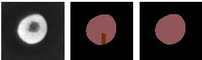

  

  For left to right: raw image, instances created after the watershed and the resulting instance after the post-proccessing. Note how the two instances of the middle image (two colors) have been merged just in one in the last image, as it should be.

• Filter instances by morphological measurements: To remove instances by the conditions based in each instance properties, which is controlled by variables inside TEST.POST_PROCESSING.MEASURE_PROPERTIES.REMOVE_BY_PROPERTIES. There are three key variables there: PROPS, VALUES and SIGN that will compose a list of conditions to remove the instances. They are list of list of conditions, for instance, the conditions can be like this: [['A'], ['B','C']]. Then, if the instance satisfies the first list of conditions, only ‘A’ in this first case (from ['A'] list), or satisfy 'B' and 'C' (from ['B','C'] list) it will be removed from the image. In each sublist all the conditions must be satisfied. The available properties are the ones that are calculated by default in TEST.POST_PROCESSING.MEASURE_PROPERTIES (explanation above). Available properties are: [circularity’, elongation’, npixels’, area’, diameter’, perimeter’, sphericity’].

  When this post-processing step is selected two .csv files will be created, one with the properties of each instance from the original image (will be placed in PATHS.RESULT_DIR.PER_IMAGE_INSTANCES path), and another with only instances that remain once this post-processing has been applied (will be placed in PATHS.RESULT_DIR.PER_IMAGE_POST_PROCESSING path). In those .csv files two more information columns will appear: a list of conditions that each instance has satisfy or not ('Satisfied', 'No satisfied' respectively), and a comment with two possible values, 'Removed' and 'Correct', telling you if the instance has been removed or not, respectively. Some of the properties follow the formulas used in MorphoLibJ library for Fiji.

  A full example of this post-processing would be the following: if you want to remove those instances that have less than 100 pixels and circularity less equal to 0.7 you should declare the above three variables as follows:

  TEST:
    POST_PROCESSING:
      MEASURE_PROPERTIES:
        REMOVE_BY_PROPERTIES:
          ENABLE: True
          PROPS:[['npixels', 'circularity']]
          VALUES: [[100, 0.7]]
          SIGN: [['lt', 'le']]
  

  You can also concatenate more restrictions and they will be applied in order. For instance, if you want to remove those instances that are bigger than an specific area, and do that before the condition described above, you can define the variables this way:

  TEST:
    POST_PROCESSING:
      MEASURE_PROPERTIES:
        REMOVE_BY_PROPERTIES:
          ENABLE: True
          PROPS:[['area'], ['npixels', 'circularity']]
          VALUES: [[500], [100, 0.7]]
          SIGN: [['gt'], ['lt', 'le']]
  

  This way, the instances will be removed by area and then by npixels and circularity.

• Voronoi tessellation: The variable TEST.POST_PROCESSING.VORONOI_ON_MASK can be enabled after the instances have been created to ensure that all instances touch each other (see Voronoi tessellation). The growth of each instance is constrained by a predefined area obtained by thresholding a channel that represents the foreground within PROBLEM.INSTANCE_SEG.DATA_CHANNEL_WEIGHTS. This channel must be one of the following: F, B, C or M (which is a legacy mask preserver to be backwards compatible with CartoCell).

The post-processing step works by performing a Voronoi tessellation using the centroid of each instance and then restricting the resulting regions to the chosen mask. This is particularly useful when you need the entire image area to be fully covered by instances with no gaps or empty spaces between them.

Metrics

During the inference phase the performance of the test data is measured using different metrics if test masks were provided (i.e. ground truth) and, consequently, DATA.TEST.LOAD_GT is True. In the case of detection, the Intersection over Union (IoU) is measured after network prediction:

• IoU: also referred as the Jaccard index, is essentially a method to quantify the percent of overlap between the target mask and the prediction output. Depending on the configuration different values are calculated (as explained in Weighting options and Metric measurement). This values can vary a lot as stated in [4].

  • Per patch: IoU is calculated for each patch separately and then averaged.

  • Reconstructed image: IoU is calculated for each reconstructed image separately and then averaged. Notice that depending on the amount of overlap/padding selected the merged image can be different than just concatenating each patch.

  • Full image: IoU is calculated for each image separately and then averaged. The results may be slightly different from the reconstructed image.

Then, after creating the final instances from the predictions, matching metrics and morphological measurements are calculated:

• Matching metrics (controlled with TEST.MATCHING_STATS): calculates precision, recall, accuracy, F1 and panoptic quality based on a defined threshold to decide whether an instance is a true positive. That threshold measures the overlap between predicted instance and its ground truth. More than one threshold can be set and it is done with TEST.MATCHING_STATS_THS. For instance, if TEST.MATCHING_STATS_THS is [0.5, 0.75] this means that these metrics will be calculated two times, one for 0.5 threshold and another for 0.75. In the first case, all instances that have more than 0.5, i.e. 50%, of overlap with their respective ground truth are considered true positives. The precision, recall and F1 are defined as follows:

  • Precision: fraction of relevant points among the retrieved points. More info here.

  • Recall: fraction of relevant points that were retrieved. More info here.

  • F1: the harmonic mean of the precision and recall. More info here.

  • Panoptic quality: defined as in Eq. 1 of Kirillov et al. “Panoptic Segmentation”, CVPR 2019.

  The code was adapted from StarDist.

• Morphological measurements (controlled by TEST.POST_PROCESSING.MEASURE_PROPERTIES): measure morphological features on each instances. The following are implemented:

  • circularity: defined as the ratio of area over the square of the perimeter, normalized such that the value for a disk equals one: (4 * PI * area) / (perimeter^2). Only measurable for 3D images (use sphericity for 3D images). While values of circularity range theoretically within the interval [0, 1], the measurements errors of the perimeter may produce circularity values above 1 (Lehmann et al., 201211).

  • elongation: the inverse of the circularity. The values of elongation range from 1 for round particles and increase for elongated particles. Calculated as: (perimeter^2)/(4 * PI * area). Only measurable for 3D images.

  • npixels: corresponds to the sum of pixels that compose an instance.

  • area: correspond to the number of pixels taking into account the image resolution (we call it area also even in a 3D image for simplicity, but that will be the volume in that case). In the resulting statistics volume will appear in that case too.

  • diameter: calculated with the bounding box and by taking the maximum value of the box in x and y axes. In 3D, z axis is also taken into account. Does not take into account the image resolution.

  • perimeter: in 3D, approximates the contour as a line through the centers of border pixels using a 4-connectivity. In 3D, it is the surface area computed using Lewiner et al. algorithm using marching_cubes and mesh_surface_area functions of scikit-image.

  • sphericity: in 3D, it is the ratio of the squared volume over the cube of the surface area, normalized such that the value for a ball equals one: (36 * PI)*((volume^2)/(perimeter^3)). Only measurable for 3D images (use circularity for 3D images).

Results

The results are placed in results folder under --result_dir directory with the --name given. Following the example, you should see that the directory /home/user/exp_results/my_3d_instance_segmentation has been created. If the same experiment is run 5 times, varying --run_id argument only, you should find the following directory tree:

Expand directory tree

my_3d_instance_segmentation/
├── config_files
│   └── 3d_instance_segmentation.yaml
├── checkpoints
│   └── my_3d_instance_segmentation_1-checkpoint-best.pth
└── results
    ├── my_3d_instance_segmentation_1
    ├── . . .
    └── my_3d_instance_segmentation_5
        ├── aug
        │   └── .tif files
        ├── charts
        │   ├── my_3d_instance_segmentation_1_*.png
        │   └── my_3d_instance_segmentation_1_loss.png
        ├── per_image
        │   ├── .tif files
        │   └── .zarr files (or.h5)
        ├── full_image
        │   └── .tif files
        ├── per_image_instances
        │   └── .tif files
        ├── per_image_instances_post_processing
        │   └── .tif files
        ├── instance_associations
        │   ├── .tif files
        │   └── .csv files
        ├── watershed
        │   ├── seed_map.tif
        │   ├── foreground.tif
        │   └── watershed.tif
        ├── train_logs
        └── tensorboard

• config_files: directory where the .yaml filed used in the experiment is stored.

  • 3d_instance_segmentation.yaml: YAML configuration file used (it will be overwrited every time the code is run).

• checkpoints, optional: directory where model’s weights are stored. Only created when TRAIN.ENABLE is True and the model is trained for at least one epoch.

  • model_weights_my_3d_instance_segmentation_1.h5, optional: checkpoint file (best in validation) where the model’s weights are stored among other information. Only created when the model is trained for at least one epoch.

  • normalization_mean_value.npy, optional: normalization mean value. Is saved to not calculate it everytime and to use it in inference. Only created if DATA.NORMALIZATION.TYPE is custom.

  • normalization_std_value.npy, optional: normalization std value. Is saved to not calculate it everytime and to use it in inference. Only created if DATA.NORMALIZATION.TYPE is custom.

• results: directory where all the generated checks and results will be stored. There, one folder per each run are going to be placed.

  • my_3d_instance_segmentation_1: run 1 experiment folder. Can contain:

    • aug, optional: image augmentation samples. Only created if AUGMENTOR.AUG_SAMPLES is True.

    • charts, optional. Only created when TRAIN.ENABLE is True and epochs trained are more or equal LOG.CHART_CREATION_FREQ:

      • my_3d_instance_segmentation_1_*.png: plot of each metric used during training.

      • my_3d_instance_segmentation_1_loss.png: loss over epochs plot.

    • per_image, optional: only created if TEST.FULL_IMG is False. Can contain:

      • .tif files, optional: reconstructed images from patches. Created when TEST.BY_CHUNKS.ENABLE is False or when TEST.BY_CHUNKS.ENABLE is True but TEST.BY_CHUNKS.SAVE_OUT_TIF is True.

      • .zarr files (or.h5), optional: reconstructed images from patches. Created when TEST.BY_CHUNKS.ENABLE is True.

    • per_image_instances:

      • .tif files: instances from reconstructed image prediction.

    • per_image_post_processing, optional: only created if a post-proccessing is enabled. Can contain:

      • .tif files: Same as per_image_instances but post-processing applied.

    • full_image, optional: only created if TEST.FULL_IMG is True. Can contain:

      • .tif files: full image predictions.

    • full_image_instances, optional: only created if TEST.FULL_IMG is True. Can contain:

      • .tif files: instances from full image prediction.

    • full_image_post_processing, optional: only created if TEST.FULL_IMG is True and a post-proccessing is enabled. Can contain:

      • .tif files: same as full_image_instances but applied post-processing.

    • as_3d_stack, optional: only created if TEST.ANALIZE_2D_IMGS_AS_3D_STACK is True. Can contain:

      • .tif files: same as full_image_instances but applied post-processing.

    • point_associations, optional: only if ground truth was provided by setting DATA.TEST.LOAD_GT. Can contain:

      • .tif files: coloured associations per each matching threshold selected to be analised (controlled by TEST.MATCHING_STATS_THS_COLORED_IMG). Green is a true positive, red is a false negative and blue is a false positive.

      • .csv files: false positives (_fp) and ground truth associations (_gt_assoc). There is a file per each matching threshold selected (controlled by TEST.MATCHING_STATS_THS).

    • watershed, optional: only if PROBLEM.INSTANCE_SEG.DATA_CHECK_MW is True. Can contain:

      • seed_map.tif: initial seeds created before growing.

      • semantic.tif: region where the watershed will run.

      • foreground.tif: foreground mask area that delimits the grown of the seeds.

    • train_logs: each row represents a summary of each epoch stats. Only avaialable if training was done.

    • tensorboard: tensorboard logs.

    • test_results_metrics.csv: a CSV file containing all the evaluation metrics obtained on each file of the test set if ground truth was provided.

Note

Here, for visualization purposes, only my_3d_instance_segmentation_1 has been described but my_3d_instance_segmentation_2, my_3d_instance_segmentation_3, my_3d_instance_segmentation_4 and my_3d_instance_segmentation_5 will follow the same structure.