Super-resolution

The goal of this workflow aims at reconstructing high-resolution (HR) images from low-resolution (LR) ones.

Input:
- LR image (single-channel or multi-channel). E.g. image with shape (500, 500, 1) (y, x, channels) in 2D or (100, 500, 500, 1) (z, y, x, channels) in 3D.
Output:
- HR image.

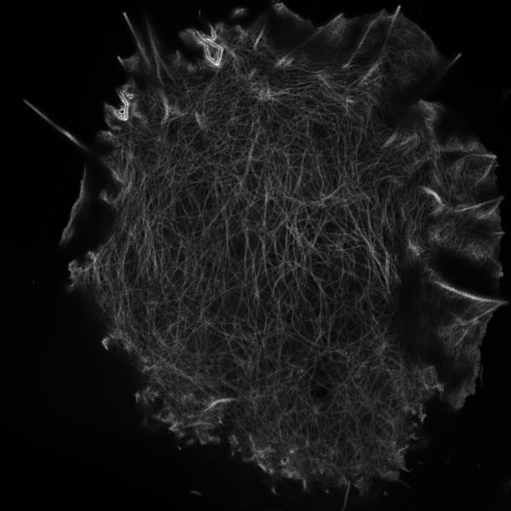
In the figure below an example of this workflow’s input is depicted to make a x2 upsampling. The images were obtained from ZeroCostDL4Mic project:

Notice that the LR image has been resized but actually that is 502x502 whereas the HR is 1004x1004.

Data preparation

To ensure the proper operation of the library the data directory tree should be something like this:

Expand directory tree

dataset/
├── train
│   ├── LR
│   │   ├── training-0001.tif
│   │   ├── training-0002.tif
│   │   ├── . . .
│   │   ├── training-9999.tif
│   └── HR
│       ├── training_0001.tif
│       ├── training_0002.tif
│       ├── . . .
│       ├── training_9999.tif
└── test
    ├── LR
    │   ├── testing-0001.tif
    │   ├── testing-0002.tif
    │   ├── . . .
    │   ├── testing-9999.tif
    └── HR
        ├── testing_0001.tif
        ├── testing_0002.tif
        ├── . . .
        ├── testing_9999.tif

Warning

Ensure that images and their corresponding masks are sorted in the same way. A common approach is to fill with zeros the image number added to the filenames (as in the example).

Configuration

Find in templates/super-resolution folder of BiaPy a few YAML configuration templates for this workflow.

Special workflow configuration

Here some special configuration options that can be selected in this workflow are described:

Upsampling is the most important variable to be set via PROBLEM.SUPER_RESOLUTION.UPSCALING. In the example above, its value is 2.
Metrics: during the inference phase the performance of the test data is measured using different metrics if test masks were provided (i.e. ground truth) and, consequently, DATA.TEST.LOAD_GT is True. In the case of super-resolution the Peak signal-to-noise ratio (PSNR) metrics is calculated when the HR image is reconstructed from individual patches.

Run

Select super-resolution workflow during the creation of a new configuration file:

https://raw.githubusercontent.com/BiaPyX/BiaPy-doc/master/source/img/gui/biapy_gui_sr.jpg

Open a terminal as described in Installation. For instance, using 2d_super-resolution.yaml template file, the code can be run as follows:

# Configuration file
job_cfg_file=/home/user/2d_super-resolution.yaml
# Path to the data directory
data_dir=/home/user/data
# Where the experiment output directory should be created
result_dir=/home/user/exp_results
# Just a name for the job
job_name=my_2d_super_resolution
# Number that should be increased when one need to run the same job multiple times (reproducibility)
job_counter=1
# Number of the GPU to run the job in (according to 'nvidia-smi' command)
gpu_number=0

sudo docker run --rm \
    --gpus "device=$gpu_number" \
    --mount type=bind,source=$job_cfg_file,target=$job_cfg_file \
    --mount type=bind,source=$result_dir,target=$result_dir \
    --mount type=bind,source=$data_dir,target=$data_dir \
    BiaPyX/biapy \
        -cfg $job_cfg_file \
        -rdir $result_dir \
        -name $job_name \
        -rid $job_counter \
        -gpu $gpu_number

Note

Note that data_dir must contain all the paths DATA.*.PATH and DATA.*.GT_PATH so the container can find them. For instance, if you want to only train in this example DATA.TRAIN.PATH and DATA.TRAIN.GT_PATH could be /home/user/data/train/x and /home/user/data/train/y respectively.

Open a terminal as described in Installation. For instance, using 2d_super-resolution.yaml template file, the code can be run as follows:

# Configuration file
job_cfg_file=/home/user/2d_super-resolution.yaml
# Where the experiment output directory should be created
result_dir=/home/user/exp_results
# Just a name for the job
job_name=my_2d_super_resolution
# Number that should be increased when one need to run the same job multiple times (reproducibility)
job_counter=1
# Number of the GPU to run the job in (according to 'nvidia-smi' command)
gpu_number=0

# Move where BiaPy installation resides
cd BiaPy

# Load the environment
conda activate BiaPy_env

python -u main.py \
    --config $job_cfg_file \
    --result_dir $result_dir  \
    --name $job_name    \
    --run_id $job_counter  \
    --gpu $gpu_number

For multi-GPU training you can call BiaPy as follows:

gpu_number="0, 1, 2"
python -u -m torch.distributed.run \
    --nproc_per_node=3 \
    main.py \
    --config $job_cfg_file \
    --result_dir $result_dir  \
    --name $job_name    \
    --run_id $job_counter  \
    --gpu $gpu_number

nproc_per_node need to be equal to the number of GPUs you are using (e.g. gpu_number length).

Results

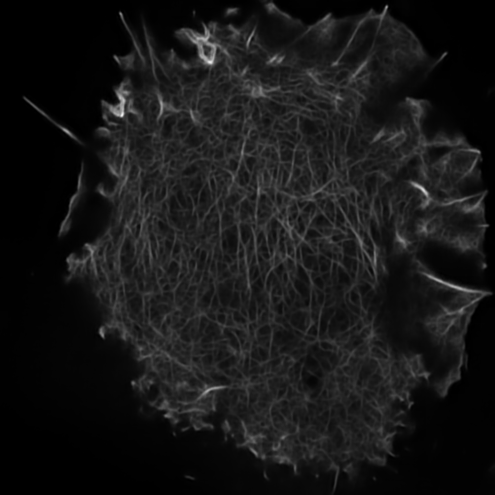
The results are placed in results folder under --result_dir directory with the --name given. An example of this workflow is depicted below:

../_images/pred_sr.png — Predicted HR image.

Here both images are of size 1004x1004.

Following the example, you should see that the directory /home/user/exp_results/my_2d_super_resolution has been created. If the same experiment is run 5 times, varying --run_id argument only, you should find the following directory tree:

Expand directory tree

my_2d_super_resolution/
├── config_files/
│   └── 2d_super-resolution.yaml
├── checkpoints
│   └── my_2d_super-resolution_1-checkpoint-best.pth
└── results
   ├── my_2d_super_resolution_1
    ├── . . .
    └── my_2d_super_resolution_5
        ├── aug
        │   └── .tif files
       ├── charts
        │   ├── my_2d_super_resolution_1_*.png
        │   ├── my_2d_super_resolution_1_loss.png
        │   └── model_plot_my_2d_super_resolution_1.png
       ├── per_image
        │   └── .tif files
        ├── train_logs
        └── tensorboard

config_files: directory where the .yaml filed used in the experiment is stored.
- 2d_super-resolution.yaml: YAML configuration file used (it will be overwrited every time the code is run)
checkpoints: directory where model’s weights are stored.
- my_2d_super-resolution_1-checkpoint-best.pth: checkpoint file (best in validation) where the model’s weights are stored among other information.
- normalization_mean_value.npy: normalization mean value (only created if DATA.NORMALIZATION.TYPE is custom). Is saved to not calculate it everytime and to use it in inference.
- normalization_std_value.npy: normalization std value (only created if DATA.NORMALIZATION.TYPE is custom). Is saved to not calculate it everytime and to use it in inference.
results: directory where all the generated checks and results will be stored. There, one folder per each run are going to be placed.
- my_2d_super_resolution_1: run 1 experiment folder.
  - aug: image augmentation samples.
  - charts:
    - my_2d_super_resolution_1_*.png: Plot of each metric used during training.
    - my_2d_super_resolution_1_loss.png: Loss over epochs plot (when training is done).
    - model_plot_my_2d_super_resolution_1.png: plot of the model.
  - per_image:
    - .tif files: reconstructed images from patches.
  - train_logs: each row represents a summary of each epoch stats. Only avaialable if training was done.
  - tensorboard: Tensorboard logs.

Note

Here, for visualization purposes, only my_2d_super_resolution_1 has been described but my_2d_super_resolution_2, my_2d_super_resolution_3, my_2d_super_resolution_4 and my_2d_super_resolution_5 will follow the same structure.