Semantic segmentation

Description of the task

The goal of this workflow is to assign a class to each pixel (or voxel) of the input image, thus producing a label image with semantic masks.

The simplest case would be binary classification, as in the figure depicted below. There, only two labels are present in the label image: black pixels (usually with value 0) represent the background, and white pixels represent the foreground (mitochondria in this case, usually labeled with 1 or 255 value).

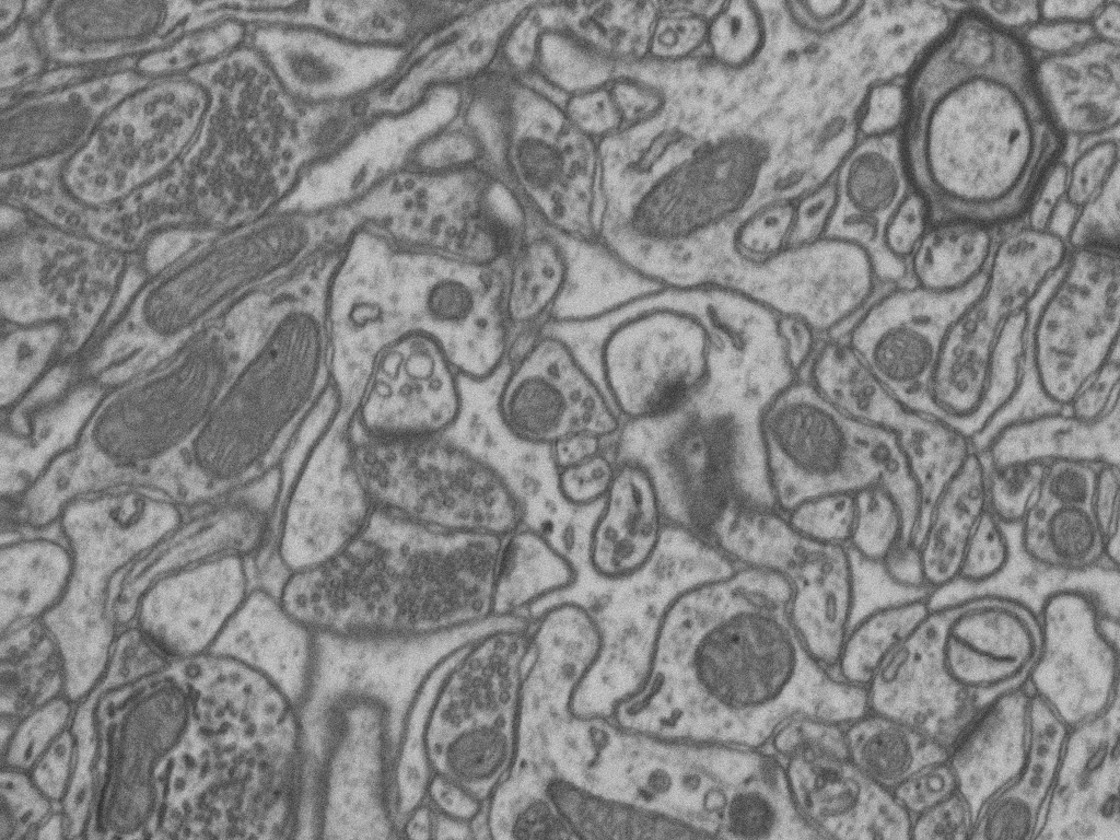
Input image (electron microscopy).

Corresponding label image with semantic masks.

If there are more than two classes, the label image is single-channel image where pixels (or voxels) of the different classes are labeled with a different integer. Below an example is depicted where 0 is background (black), 1 are outlines (pink) and 2 nuclei (light blue).

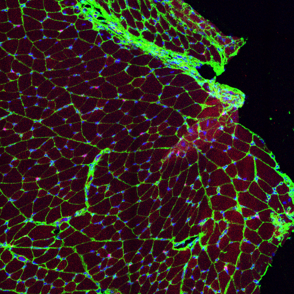
Input image (fluorescence microscopy).

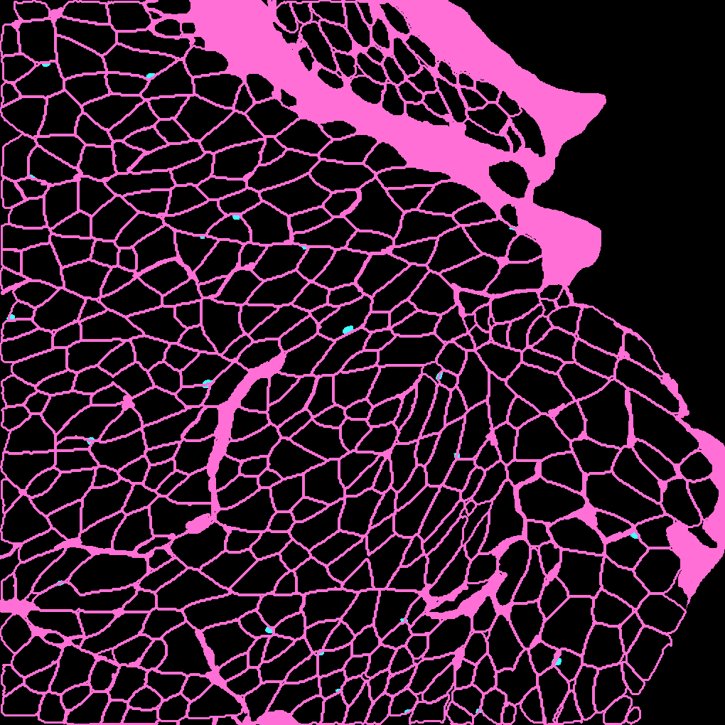
Corresponding label image with semantic masks.

Inputs and outputs

The semantic segmentation workflows in BiaPy expect a series of folders as input:

• Training Raw Images: A folder that contains the unprocessed (single-channel or multi-channel) images that will be used to train the model.

  Expand to see how to configure

  GUIGoogle Colab / NotebooksYAML configuration file

  In the current BiaPy GUI, this option is defined through the Wizard questions. Alternatively, you can edit the DATA.TRAIN.PATH in your YAML file before clicking Run Workflow and loading that YAML file.

• Training Label Images: A folder that contains the semantic label (single-channel) images for training. Ensure the number and dimensions match the training raw images.

  Expand to see how to configure

  GUIGoogle Colab / NotebooksYAML configuration file

  In the current BiaPy GUI, this option is defined through the Wizard questions. Alternatively, you can edit the DATA.TRAIN.GT_PATH in your YAML file before clicking Run Workflow and loading that YAML file.

• [Optional] Test Raw Images: A folder that contains the images to evaluate the model's performance.
  Expand to see how to configure

  GUIGoogle Colab / NotebooksYAML configuration file

  In the current BiaPy GUI, this option is defined through the Wizard questions. Alternatively, you can edit the DATA.TEST.PATH in your YAML file before clicking Run Workflow and loading that YAML file.

• [Optional] Test Label Images: A folder that contains the semantic label images for testing. Again, ensure their count and sizes align with the test raw images.
  Expand to see how to configure

  GUIGoogle Colab / NotebooksYAML configuration file

  In the current BiaPy GUI, this option is defined through the Wizard questions. Alternatively, you can edit the DATA.TEST._GT_PATH in your YAML file before clicking Run Workflow and loading that YAML file.

Upon successful execution, a directory will be generated with the segmentation results. Both probability maps and label images will be available there. Therefore, you will need to define:

• Output Folder: A designated path to save the segmentation outcomes.

  Expand to see how to configure

  GUIGoogle Colab / NotebooksCommand line

  Under Run Workflow, click on the Browse button of Output folder to save the results:

  

BiaPy input and output folders for semantic segmentation.

Data structure

To ensure the proper operation of the library, the data directory tree should be something like this:

dataset/
├── train
│   ├── raw
│   │   ├── training-0001.tif
│   │   ├── training-0002.tif
│   │   ├── . . .
│   │   └── training-9999.tif
│   └── label
│       ├── training_groundtruth-0001.tif
│       ├── training_groundtruth-0002.tif
│       ├── . . .
│       └── training_groundtruth-9999.tif
└── test
    ├── raw
    │   ├── testing-0001.tif
    │   ├── testing-0002.tif
    │   ├── . . .
    │   └── testing-9999.tif
    └── label
        ├── testing_groundtruth-0001.tif
        ├── testing_groundtruth-0002.tif
        ├── . . .
        └── testing_groundtruth-9999.tif

In this example, the raw training images are under dataset/train/raw/ and their corresponding labels are under dataset/train/label/, while the raw test images are under dataset/test/raw/ and their corresponding labels are under dataset/test/label/. This is just an example, you can name your folders as you wish as long as you set the paths correctly later.

Note

Ensure that images and their corresponding masks are sorted in the same way. A common approach is to fill with zeros the image number added to the filenames (as in the example).

Example datasets

Below is a list of publicly available datasets that are ready to be used in BiaPy for semantic segmentation:

Example dataset	Image dimensions	Link to data
Electron Microscopy Dataset (EPFL - CVLAB)	2D	fibsem_epfl.zip
Electron Microscopy Dataset (EPFL - CVLAB)	3D	lucchi3D.zip

Minimal configuration

Apart from the input and output folders, there are a few basic parameters that always need to be specified in order to run a semantic segmentation workflow in BiaPy. Depending on the parameter, they can be defined through the GUI Wizard, in the code-free notebooks, or by editing the YAML configuration file.

Experiment name

Also known as “model name” or “job name”, this will be the name of the current experiment you want to run, so it can be differenciated from other past and future experiments.

Expand to see how to configure

GUIGoogle Colab / NotebooksCommand line

Under Run Workflow, type the name you want for the job in the Job name field:

Note

Use only my_model -style, not my-model (Use “_” not “-“). Do not use spaces in the name. Avoid using the name of an existing experiment/model/job (saved in the same result folder) as it will be overwritten..

Data management

Validation Set

With the goal to monitor the training process, it is common to use a third dataset called the “Validation Set”. This is a subset of the whole dataset that is used to evaluate the model’s performance and optimize training parameters. This subset will not be directly used for training the model, and thus, when applying the model to these images, we can see if the model is learning the training set’s patterns too specifically or if it is generalizing properly.

Graphical description of data partitions in BiaPy.

To define such set, there are two options:

• Validation proportion/percentage: Select a proportion (or percentage) of your training dataset to be used to validate the network during the training. Usual values are 0.1 (10%) or 0.2 (20%), and the samples of that set will be selected at random.

  Expand to see how to configure

  GUIGoogle Colab / NotebooksYAML configuration file

  In the current BiaPy GUI, this option is configured by editing the DATA.VAL.SPLIT_TRAIN in your YAML file before clicking Run Workflow and loading that YAML file.

• Validation paths: Similar to the training and test sets, you can select two folders with the validation raw and label images:

  • Validation Raw Images: A folder that contains the unprocessed (single-channel or multi-channel) images that will be used to select the best model during training.

    Expand to see how to configure

    GUIGoogle Colab / NotebooksYAML configuration file

    In the current BiaPy GUI, this option is configured by editing the DATA.VAL.PATH in your YAML file before clicking Run Workflow and loading that YAML file.

  • Validation Label Images: A folder that contains the semantic label (single-channel) images for validation. Ensure the number and dimensions match the validation raw images.

    Expand to see how to configure

    GUIGoogle Colab / NotebooksYAML configuration file

    In the current BiaPy GUI, this option is configured by editing the DATA.VAL.GT_PATH in your YAML file before clicking Run Workflow and loading that YAML file.

Test ground-truth

Do you have labels for the test set? This is a key question so BiaPy knows if your test set will be used for evaluation in new data (unseen during training) or simply produce predictions on that new data. All supervised workflows contain a parameter to specify this aspect.

Expand to see how to configure

GUIGoogle Colab / NotebooksYAML configuration file

In the current BiaPy GUI, this option is defined through the Wizard questions. Alternatively, you can edit the DATA.TEST.LOAD_GT in your YAML file before clicking Run Workflow and loading that YAML file.

Basic training parameters

At the core of each BiaPy workflow there is a deep learning model. Although we try to simplify the number of parameters to tune, these are the basic parameters that need to be defined for training a semantic segmentation workflow:

• Number of classes: The number of segmentation labels, including the background, whose label is usually set to 0. For instance, if you are doing foreground vs background semantic segmentation, the number of classes will be 2 (one for foreground and one for background).

  Expand to see how to configure

  GUIGoogle Colab / NotebooksYAML configuration file

  In the current BiaPy GUI, this option is configured by editing the MODEL.N_CLASSES in your YAML file before clicking Run Workflow and loading that YAML file.

• Number of input channels: The number of channels of your raw images (grayscale = 1, RGB = 3). Notice the dimensionality of your images (2D/3D) is set by default depending on the workflow template you select.

  Expand to see how to configure

  GUIGoogle Colab / NotebooksYAML configuration file

  In the current BiaPy GUI, this option is configured by editing the DATA.PATCH_SIZE in your YAML file before clicking Run Workflow and loading that YAML file.

• Number of epochs: This number indicates how many rounds the network will be trained. On each round, the network usually sees the full training set. The value of this parameter depends on the size and complexity of each dataset. You can start with something like 100 epochs and tune it depending on how fast the loss (error) is reduced.

  Expand to see how to configure

  GUIGoogle Colab / NotebooksYAML configuration file

  In the current BiaPy GUI, this option is configured by editing the TRAIN.EPOCHS in your YAML file before clicking Run Workflow and loading that YAML file.

• Patience: This is a number that indicates how many epochs you want to wait without the model improving its results in the validation set to stop training. Again, this value depends on the data you’re working on, but you can start with something like 20.

  Expand to see how to configure

  GUIGoogle Colab / NotebooksYAML configuration file

  In the current BiaPy GUI, this option is configured by editing the TRAIN.PATIENCE in your YAML file before clicking Run Workflow and loading that YAML file.

For improving performance, other advanced parameters can be optimized, for example, the model’s architecture. The architecture assigned as default is the U-Net, as it is effective in semantic segmentation tasks. This architecture allows a strong baseline, but further exploration could potentially lead to better results.

Note

Once the parameters are correctly assigned, the training phase can be executed. Note that to train large models effectively the use of a GPU (Graphics Processing Unit) is essential. This hardware accelerator performs parallel computations and has larger RAM memory compared to the CPUs, which enables faster training times.

How to run

BiaPy offers different options to run workflows depending on your degree of computer expertise. Select whichever is more approppriate for you:

GUIGoogle ColabDockerCommand line

In the BiaPy GUI, click on the Wizard, then follow the next instructions to select the semantic segmentation workflow:

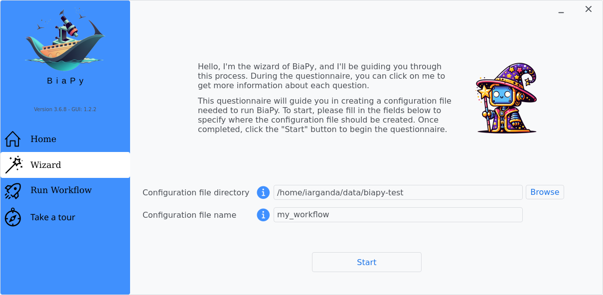
Step 1: Choose a folder and file name to store your workflow configuration file, then click "Start".

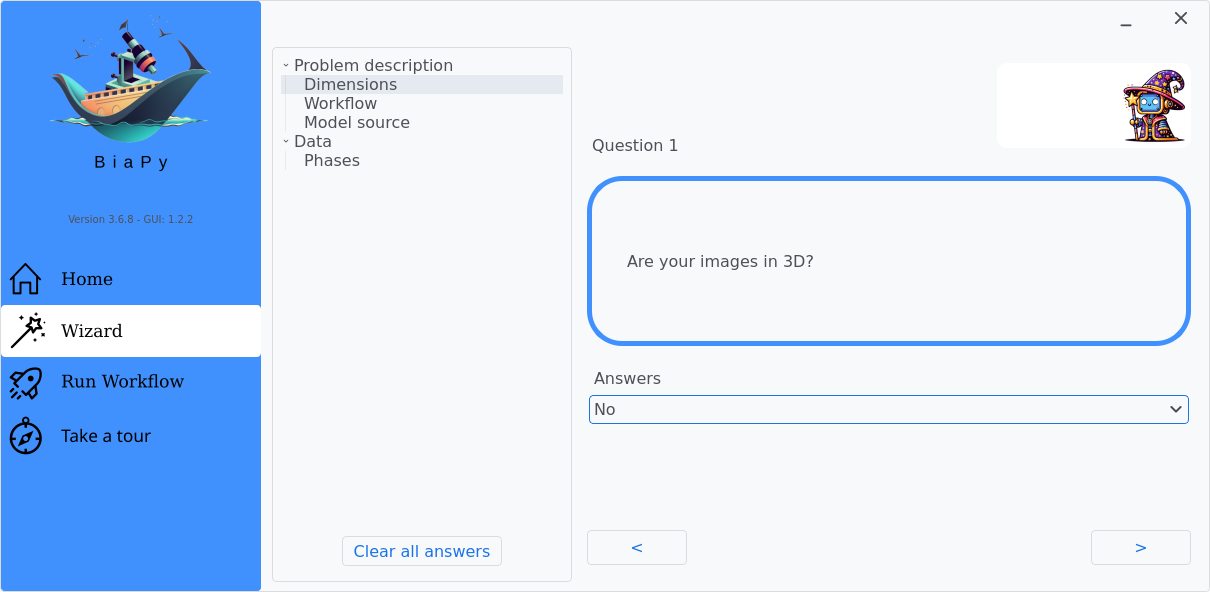
Step 2: Under Question 1, select the answer that best fits with your data dimensionality.

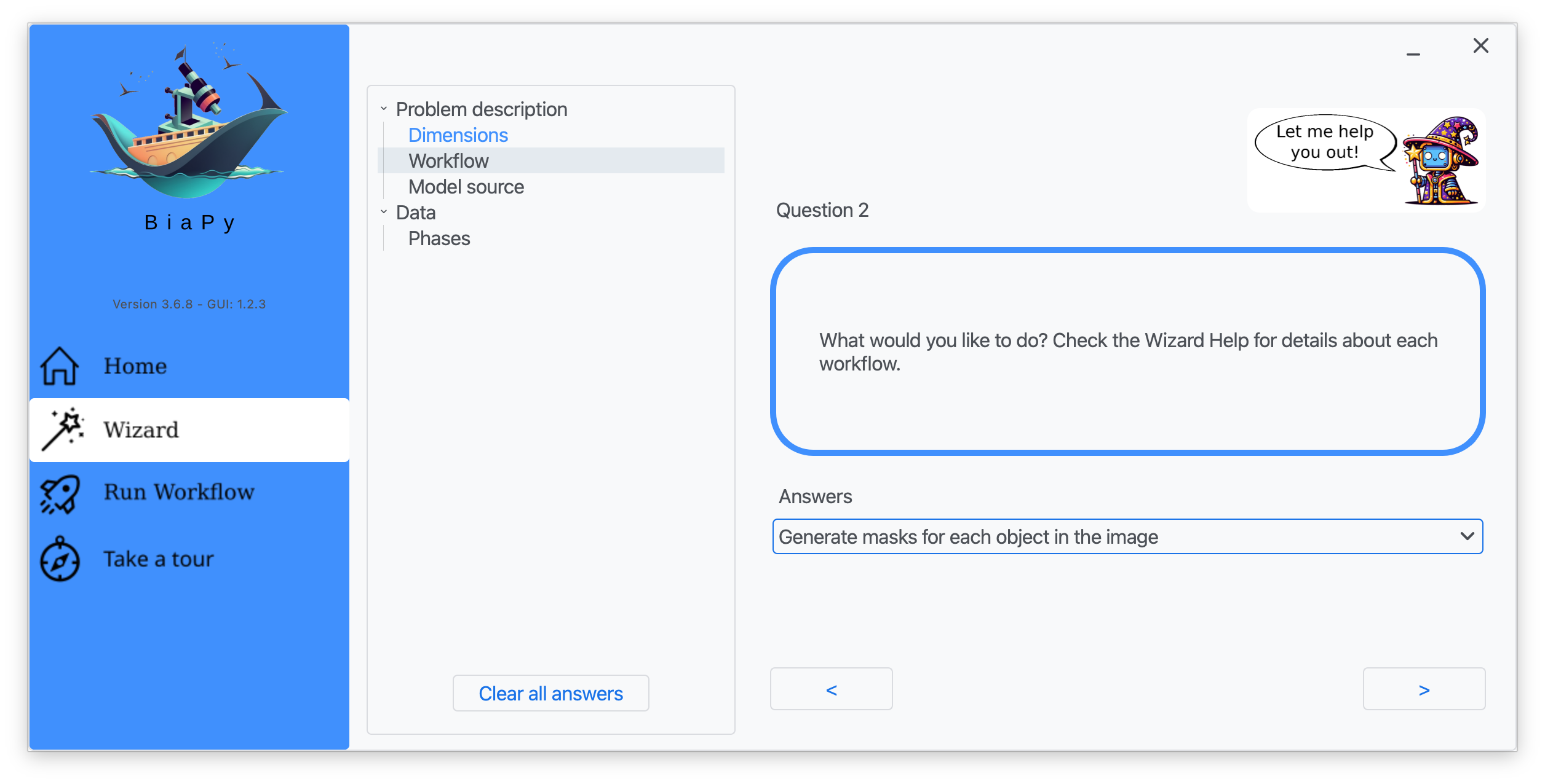
Step 3: Under Question 2, select the answer "Generate masks for each object in the image".

Previous Next

After that, you will be able to edit the parameters of the workflow and run it.

Note

BiaPy’s GUI requires that all data and configuration files reside on the same machine where the GUI is being executed.

For a full example on how to configure a semantic segmentation workflow in BiaPy GUI, watch our semantic segmentation demo video:

Tip

If you need additional help, watch BiaPy’s GUI walkthrough video.

Templates

In the templates/semantic_segmentation folder of BiaPy, you will find a few YAML configuration templates for this workflow.

[Advanced] Special workflow configuration

Note

This section is recommended for experienced users only to improve the performance of their workflows. When in doubt, do not hesitate to check our FAQ & Troubleshooting or open a question in the image.sc discussion forum.

Advanced Parameters

Many of the parameters of our workflows are set by default to values that work commonly well. However, it may be needed to tune them to improve the results of the workflow. For instance, you may modify the following parameters

• Model architecture: Select the architecture of the deep neural network used as backbone of the pipeline. Options: U-Net, Residual U-Net, Attention U-Net, SEUNet, MultiResUNet, ResUNet++, UNETR-Mini, UNETR-Small, UNETR-Base, ResUNet SE and U-NeXt V1. Default value: U-Net.

• Batch size: This parameter defines the number of patches seen in each training step. Reducing or increasing the batch size may slow or speed up your training, respectively, and can influence network performance. Common values are 4, 8, 16, etc.

• Patch size: Input the size of the patches use to train your model (length in pixels in X and Y). The value should be smaller or equal to the dimensions of the image. The default value is 256 in 2D, i.e. 256x256 pixels.

• Optimizer: Select the optimizer used to train your model. Options: ADAM, ADAMW, Stochastic Gradient Descent (SGD). ADAM usually converges faster, while ADAMW provides a balance between fast convergence and better handling of weight decay regularization. SGD is known for better generalization. Default value: ADAMW.

• Initial learning rate: Input the initial value to be used as learning rate. If you select ADAM as optimizer, this value should be around 10e-4.

• Learning rate scheduler: Select to adjust the learning rate between epochs. The current options are “Reduce on plateau”, “One cycle”, “Warm-up cosine decay” or no scheduler.

• Test time augmentation (TTA): Select to apply augmentation (flips and rotations) at test time. It usually provides more robust results but uses more time to produce each result. By default, no TTA is peformed.

Output

The output of a semantic segmentation workflow can be:

• Single-channel image, when DATA.TEST.ARGMAX_TO_OUTPUT is True, with each class labeled with an integer.

• Multi-channel image, when DATA.TEST.ARGMAX_TO_OUTPUT is False, with the same number of channels as classes, and the same pixel in each channel will be the probability (in [0-1] range) of being of the class that represents that channel number. For instance, with 3 classes, e.g. background, mitochondria and contours, the fist channel will represent background, the second mitochondria and the last the contours.

Data loading

If you want to select DATA.EXTRACT_RANDOM_PATCH you can also set DATA.PROBABILITY_MAP to create a probability map so the patches extracted will have a high probability of having an object in the middle of it. Useful to avoid extracting patches which no foreground class information. That map will be saved in PATHS.PROB_MAP_DIR. Furthermore, in PATHS.DA_SAMPLES path, i.e. aug folder by default (see Results), two more images will be created so you can check how this probability map is working. These images will have painted a blue square and a red point in its middle, which correspond to the patch area extracted and the central point selected respectively. One image will be named as mark_x and the other one as mark_y, which correspond to the input image and ground truth respectively.

Metrics

During the inference phase the performance of the test data is measured using different metrics if test masks were provided (i.e. ground truth) and, consequently, DATA.TEST.LOAD_GT is True. In the case of semantic segmentation the Intersection over Union (IoU) metrics is calculated after the network prediction. This metric, also referred as the Jaccard index, is essentially a method to quantify the percent of overlap between the target mask and the prediction output. Depending on the configuration different values are calculated (as explained in Weighting options and Metric measurement). This values can vary a lot as stated in [4].

• Per patch: IoU is calculated for each patch separately and then averaged.

• Reconstructed image: IoU is calculated for each reconstructed image separately and then averaged. Notice that depending on the amount of overlap/padding selected the merged image can be different than just concatenating each patch.

• Full image: IoU is calculated for each image separately and then averaged. The results may be slightly different from the reconstructed image.

Post-processing

Only applied to 3D images (e.g. PROBLEM.NDIM is 2D or TEST.ANALIZE_2D_IMGS_AS_3D_STACK is True). There are the following options:

• Z-filtering: to apply a median filtering in z axis. Useful to maintain class coherence across 3D volumes. Enable it with TEST.POST_PROCESSING.Z_FILTERING and use TEST.POST_PROCESSING.Z_FILTERING_SIZE for the size of the median filter.

• YZ-filtering: to apply a median filtering in y and z axes. Useful to maintain class coherence across 3D volumes that can work slightly better than Z-filtering. Enable it with TEST.POST_PROCESSING.YZ_FILTERING and use TEST.POST_PROCESSING.YZ_FILTERING_SIZE for the size of the median filter.

Results

The results are placed in results folder under --result_dir directory with the --name given. An example of this workflow is depicted below:

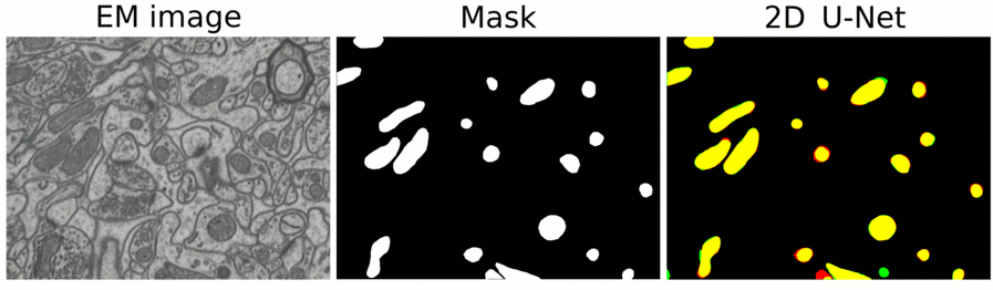
Example of semantic segmentation model predictions. From left to right: input image, its mask and the overlap between the mask and the model’s output binarized.

Following the example, you should see that the directory /home/user/exp_results/my_2d_semantic_segmentation has been created. If the same experiment is run 5 times, varying --run_id argument only, you should find the following directory tree:

Expand directory tree

my_2d_semantic_segmentation/
├── config_files
│   └── my_2d_semantic_segmentation_1.yaml
├── checkpoints
│   └── my_2d_semantic_segmentation_1-checkpoint-best.pth
└── results
    ├── my_2d_semantic_segmentation_1
    ├── . . .
    └── my_2d_semantic_segmentation_5
        ├── aug
        │   └── .tif files
        ├── charts
        │   ├── my_2d_semantic_segmentation_1_*.png
        │   └── my_2d_semantic_segmentation_1_loss.png
        ├── per_image
        │   ├── .tif files
        │   └── .zarr files (or.h5)
        ├── per_image_binarized
        │   └── .tif files
        ├── full_image
        │   └── .tif files
        ├── full_image_binarized
        │   └── .tif files
        ├── full_post_processing
        │   └── .tif files
        ├── tensorboard
        └── train_logs

• config_files: directory where the .yaml filed used in the experiment is stored.

  • my_2d_semantic_segmentation.yaml: YAML configuration file used (it will be overwrited every time the code is run)

• checkpoints, optional: directory where model’s weights are stored. Only created when TRAIN.ENABLE is True and the model is trained for at least one epoch.

  • my_2d_semantic_segmentation_1-checkpoint-best.pth, optional: checkpoint file (best in validation) where the model’s weights are stored among other information. Only created when the model is trained for at least one epoch.

  • normalization_mean_value.npy, optional: normalization mean value. Is saved to not calculate it everytime and to use it in inference. Only created if DATA.NORMALIZATION.TYPE is custom.

  • normalization_std_value.npy, optional: normalization std value. Is saved to not calculate it everytime and to use it in inference. Only created if DATA.NORMALIZATION.TYPE is custom.

• results: directory where all the generated checks and results will be stored. There, one folder per each run are going to be placed.

  • my_2d_semantic_segmentation_1: run 1 experiment folder. Can contain:

    • aug, optional: image augmentation samples. Only created if AUGMENTOR.AUG_SAMPLES is True.

    • charts, optional: only created when TRAIN.ENABLE is True and epochs trained are more or equal LOG.CHART_CREATION_FREQ. Can contain:

      • my_2d_semantic_segmentation_1_*.png: plot of each metric used during training.

      • my_2d_semantic_segmentation_1_loss.png: loss over epochs plot.

    • per_image, optional: only created if TEST.FULL_IMG is False. Can contain:

      • .tif files, optional: reconstructed images from patches. Created when TEST.BY_CHUNKS.ENABLE is False or when TEST.BY_CHUNKS.ENABLE is True but TEST.BY_CHUNKS.SAVE_OUT_TIF is True.

      • .zarr files (or.h5), optional: reconstructed images from patches. Created when TEST.BY_CHUNKS.ENABLE is True.

    • per_image_binarized, optional: only created if TEST.FULL_IMG is False. Can contain:

      • .tif files: Same as per_image but with the images binarized.

    • full_image, optional: only created if TEST.FULL_IMG is True. Can contain:

      • .tif files: full image predictions.

    • full_image_binarized:

      • .tif files: Same as full_image but with the image binarized.

    • tensorboard: Tensorboard logs.

    • train_logs: each row represents a summary of each epoch stats. Only avaialable if training was done.

    • test_results_metrics.csv: a CSV file containing all the evaluation metrics obtained on each file of the test set if ground truth was provided.

Note

Here, for visualization purposes, only my_2d_semantic_segmentation_1 has been described but my_2d_semantic_segmentation_2, my_2d_semantic_segmentation_3, my_2d_semantic_segmentation_4 and my_2d_semantic_segmentation_5 will follow the same structure.