Self-supervision

The idea of this workflow is to pretrain the backbone model by solving a so-called pretext task without labels. This way, the model learns a representation that can be later transferred to solve a downstream task in a labeled (but smaller) dataset. In BiaPy we adopt two pretext tasks that you will need to choose with pretext_task variable below (controlled with PROBLEM.SELF_SUPERVISED.PRETEXT_TASK). The pretext tasks implemented in BiaPy are these:

• crappify: To recover a worstened version of the input image as in ([FBPTGonzalezM+22]).

• masking: Random patches of the input image are masked and the network needs to reconstruct the missing pixels ([HCX+22]).

• Input:

  • Image.

• Output:

  • Pretrained model.

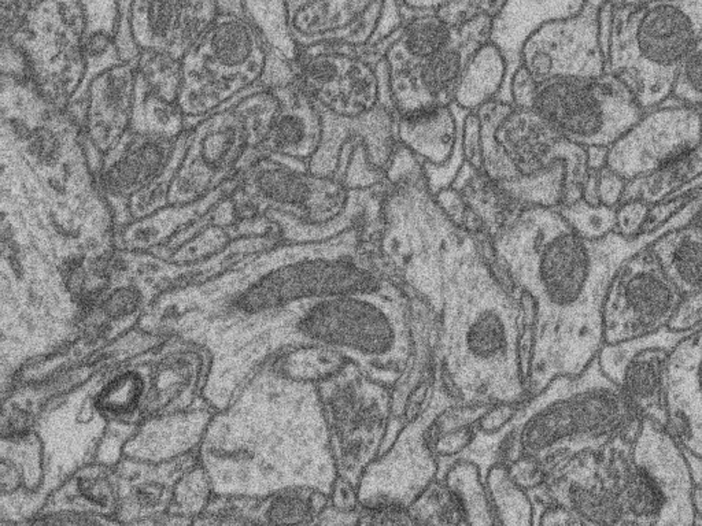
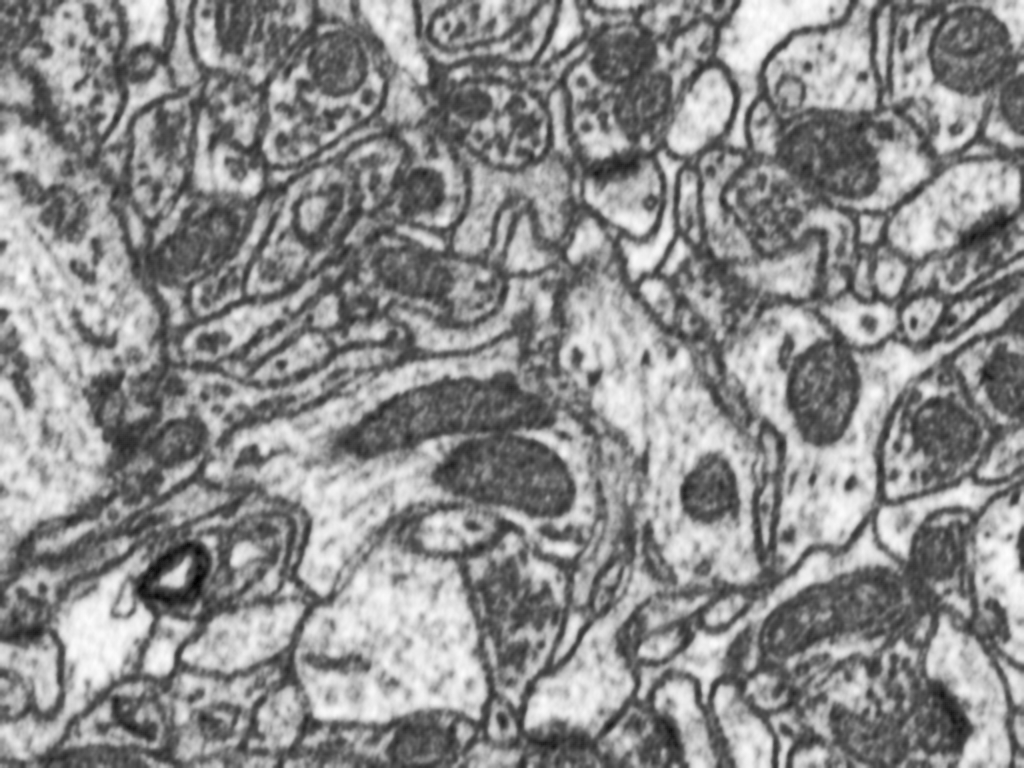
In the figure below an example of crappify pretext task input images are depicted:

Input image’s worstened version.

Input image.

Data preparation

To ensure the proper operation of the library the data directory tree should be something like this:

dataset/
├── train
│   └── x
│       ├── training-0001.tif
│       ├── training-0002.tif
│       ├── . . .
│       └── training-9999.tif
└── test
    └── x
        ├── testing-0001.tif
        ├── testing-0002.tif
        ├── . . .
        └── testing-9999.tif

Problem resolution

CrappifyMasking

Firstly, a pre-processing step is done where the input images are worstened by adding Gaussian noise and downsampling and upsampling them so the resolution gets worsen. This way, the images are stored in DATA.TRAIN.SSL_SOURCE_DIR, DATA.VAL.SSL_SOURCE_DIR and DATA.TEST.SSL_SOURCE_DIR for train, validation and test data respectively. This way, the model will be input with the worstened version of images and will be trained to map it to its good version.

After this training, the model should have learned some features of the images, which will be a good starting point in another training process. This way, if you re-train the model loading those learned model’s weigths, which can be done enabling MODEL.LOAD_CHECKPOINT if you call BiaPy with the same --name option or setting PATHS.CHECKPOINT_FILE variable to point the file directly otherwise, the training process will be easier and faster than training from scratch.

Configuration file

Find in templates/self-supervised folder of BiaPy a few YAML configuration templates for this workflow.

Special workflow configuration

Here some special configuration options that can be selected in this workflow are described:

• Metrics: during the inference phase the performance of the test data is measured using different metrics if test masks were provided (i.e. ground truth) and, consequently, DATA.TEST.LOAD_GT is enabled. In the case of super-resolution the Peak signal-to-noise ratio (PSNR) metrics is calculated when the worstened image is reconstructed from individual patches.

Run

Command lineDockerGoogle Colab

Open a terminal as described in Installation. For instance, using 2d_self-supervised.yaml template file, the code can be run as follows:

# Configuration file
job_cfg_file=/home/user/2d_self-supervised.yaml
# Where the experiment output directory should be created
result_dir=/home/user/exp_results
# Just a name for the job
job_name=my_2d_self-supervised
# Number that should be increased when one need to run the same job multiple times (reproducibility)
job_counter=1
# Number of the GPU to run the job in (according to 'nvidia-smi' command)
gpu_number=0

# Move where BiaPy installation resides
cd BiaPy

# Load the environment
conda activate BiaPy_env
source $CONDA_PREFIX/etc/conda/activate.d/env_vars.sh

python -u main.py \
    --config $job_cfg_file \
    --result_dir $result_dir  \
    --name $job_name    \
    --run_id $job_counter  \
    --gpu $gpu_number

For multi-GPU training you can call BiaPy as follows:

gpu_number="0, 1, 2"
python -u -m torch.distributed.run \
    --nproc_per_node=3 \
    main.py \
    --config $job_cfg_file \
    --result_dir $result_dir  \
    --name $job_name    \
    --run_id $job_counter  \
    --gpu $gpu_number

nproc_per_node need to be equal to the number of GPUs you are using (e.g. gpu_number length).

Results

The results are placed in results folder under --result_dir directory with the --name given. An example of this workflow is depicted below:

Predicted image.

Original input image.

Following the example, you should see that the directory /home/user/exp_results/my_2d_self-supervised has been created. If the same experiment is run 5 times, varying --run_id argument only, you should find the following directory tree:

my_2d_self-supervised/
├── config_files/
│   └── my_2d_self-supervised.yaml
├── checkpoints
│   └── my_2d_self-supervised_1-checkpoint-best.pth
└── results
    ├── my_2d_self-supervised_1
    ├── . . .
    └── my_2d_self-supervised_5
        ├── aug
        │   └── .tif files
        ├── charts
        │   ├── my_2d_self-supervised_1_*.png
        │   ├── my_2d_self-supervised_1_loss.png
        │   └── model_plot_my_2d_self-supervised_1.png
        ├── MAE_checks
        │   └── .tif files
        ├── per_image
        │   └── .tif files
        ├── tensorboard
        └── train_logs

• config_files: directory where the .yaml filed used in the experiment is stored.

  • my_2d_self-supervised.yaml: YAML configuration file used (it will be overwrited every time the code is run).

• checkpoints: directory where model’s weights are stored.

  • my_2d_self-supervised_1-checkpoint-best.pth: checkpoint file (best in validation) where the model’s weights are stored among other information.

  • normalization_mean_value.npy: normalization mean value (only created if DATA.NORMALIZATION.TYPE is custom). Is saved to not calculate it everytime and to use it in inference.

  • normalization_std_value.npy: normalization std value (only created if DATA.NORMALIZATION.TYPE is custom). Is saved to not calculate it everytime and to use it in inference.

• results: directory where all the generated checks and results will be stored. There, one folder per each run are going to be placed.

  • my_2d_self-supervised_1: run 1 experiment folder.

    • aug: image augmentation samples.

    • charts:

      • my_2d_self-supervised_1_*.png: Plot of each metric used during training.

      • my_2d_self-supervised_1_loss.png: Loss over epochs plot (when training is done).

      • model_plot_my_2d_self-supervised_1.png: plot of the model.

    • MAE_checks: MAE predictions. Only available if PROBLEM.SELF_SUPERVISED.PRETEXT_TASK is masking.

      • *_original.tif: Original image.

      • *_masked.tif: Masked image inputed to the model.

      • *_reconstruction.tif: Reconstructed image.

      • *_reconstruction_and_visible.tif: Reconstructed image with the visible parts copied.

    • per_image:

      • .tif files: reconstructed images from patches.

    • tensorboard: Tensorboard logs.

    • train_logs: each row represents a summary of each epoch stats. Only avaialable if training was done.

Note

Here, for visualization purposes, only my_2d_self-supervised_1 has been described but my_2d_self-supervised_2, my_2d_self-supervised_3, my_2d_self-supervised_4 and my_2d_self-supervised_5 will follow the same structure.