CartoCell, a high-throughput pipeline for accurate 3D image analysis (Paper)

About this tutorial

This tutorial describes how to create a custom 3D instance segmentation workflow to reproduce the results published in “CartoCell, a high-content pipeline for 3D image analysis, unveils cell morphology patterns in epithelia” (Cell Report Methods, 2023) using BiaPy.

Note

If you are mainly interested in applying CartoCell’s pretrained models (without reproducing all training phases), go directly to Model testing in the latest BiaPy workflow.

Graphical abstract of CartoCell (2023).

This workflow targets 3D epithelial cysts acquired with confocal microscopy. The segmented cells need to be in direct contact to study their packaging and organization.

Example of cyst raw image (CartoCell dataset).

Corresponding cyst label image (CartoCell dataset).

CartoCell overview

CartoCell follows a multi-phase pipeline to, given an initial training dataset of 21 3D labeled cysts, automatically segment hundreds of cysts at low resolution with enough quality to perform cell organization and packaging analysis. The five phases of CartoCell are briefly explained in the following tabs:

Phase 1Phase 2Phase 3Phase 4Phase 5

A small dataset of 21 cysts, stained with cell outlines markers, was acquired at high-resolution in a confocal microscope. Next, the individual cell instances were semi-automatically segmented and manually curated. The high-resolution images from Phase 1 provide the accurate and realistic set of data necessary for the following steps.

Data preparation

All data needed in this tutorial is accessible through Zenodo here. Download and unzip the CartoCell.zip file (185.7 MB). Once unzipped, you should find the following directory tree:

CartoCell/
├── train_M1
│   ├── x
│   │   ├── Cyst 4d filt 2po Pha,Bcat,DAPI 02.08.19 40x POC 3 Z6.tif
│   │   ├── Cyst 4d filt 2po Pha,Bcat,DAPI 02.08.19 40x Z4.5 4a.tif
│   │   ├── . . .
│   │   └── cyst 7d filt 3po pha bcat dapi 15.07.19 40x z4.5 4a.tif
│   └── y
│       ├── Cyst 4d filt 2po Pha,Bcat,DAPI 02.08.19 40x POC 3 Z6.tif
│       ├── Cyst 4d filt 2po Pha,Bcat,DAPI 02.08.19 40x Z4.5 4a.tif
│       ├── . . .
│       └── cyst 7d filt 3po pha bcat dapi 15.07.19 40x z4.5 4a.tif
├── validation
│   ├── x
│   │   ├── CYST 7d Filt 3well Pha,Bcat,DAPI 40x Z4 15.7.19 3a.tif
│   │   └── cyst 4d fil 3well Pha,bcat,dapi 02.08.19 40x Z5 12a.tif
│   └── y
│       ├── CYST 7d Filt 3well Pha,Bcat,DAPI 40x Z4 15.7.19 3a.tif
│       └── cyst 4d fil 3well Pha,bcat,dapi 02.08.19 40x Z5 12a.tif
├── train_M2
│   ├── x
│   │   ├── 10d.1B.26.2.tif
│   │   ├── 10d.1B.29.1.tif
│   │   ├── . . .
│   │   └── control_7d.3HX3.1HX1.C.9.3.tif
│   └── y
│       ├── 10d.1B.26.2.tif
│       ├── 10d.1B.29.1.tif
│       ├── . . .
│       └── control_7d.3HX3.1HX1.C.9.3.tif
└── test
    ├── x
    │   ├── 10d.1B.10.1.tif
    │   ├── 10d.1B.10.2.tif
    │   ├── . . .
    │   └── 7d.4C.8_2.tif
    └── y
        ├── 10d.1B.10.1.tif
        ├── 10d.1B.10.2.tif
        ├── . . .
        └── 7d.4C.8_2.tif

More specifically, the data you need on each phase is as follows:

• Phase 2: folders train_M1 (19 volumes) and validation (2 volumes) to train the initial model (model M1).

• Phases 3 and 4: folder train_M2 (293 volumes) to be segmented with model M1 (phase 3) and then train model M2 (phase 4).

• Phase 5: test (60 volumes) to run the inference using our pretrained model M2 on unseen data.

Reproducing published results (legacy version)

BiaPy, the library behind CartoCell, has undergone many changes since the CartoCell paper was published. Here you have the instructions to reproduce exactly the CartoCell pipeline using the same version of BiaPy available at the time of publication.

Note

CartoCell can also be executed using the latest version of BiaPy (see instructions below). These steps are only needed to use the exact same code and configuration used at the time of publication.

Configure environment for old BiaPy version

To reproduce the exact pipeline published with our manuscript, you need to configure BiaPy to use the code version associated with the publication. To do so, the easiest way is to configure a Conda environment from the command line as follows:

# Create environment called "CartoCell_env" using Python v3.10.11
conda create -n CartoCell_env python=3.10.11

# Activate environment
conda activate CartoCell_env

# Install dependencies
conda install scikit-image==0.20.0 scikit-learn==1.2.2 tqdm==4.65.0 pandas==1.5.3
conda install imgaug==0.4.0 yacs==0.1.6 pydot

pip install fill-voids

conda install -c conda-forge tensorflow-gpu==2.11.1 edt==2.3.1

Model training

The training of model M1 and model M2 is essentially the same, only the input dataset changes. To train either model, you have two options: via command line or using Google Colab.

Command lineGoogle Colab

You can reproduce the exact results of our manuscript via the command line using the cartocell_training.yaml configuration file.

• In case you want to reproduce the training of our model M1 (from phase 2), you will need to modify the DATA.TRAIN.PATH and DATA.TRAIN.GT_PATH with the paths to the folders containing the raw images and their corresponding labels, that is to say, with the paths of train_M1/x and train_M1/y respectively.

• In case you want to reproduce the training of our model M2 (from phase 4), you will need to modify the DATA.TRAIN.PATH and DATA.TRAIN.GT_PATH as above but now using the paths of train_M2/x and train_M2/y.

For the validation data, for both model M1 and model M2, you will need to modify DATA.VAL.PATH and DATA.VAL.GT_PATH with the paths of validation/x and validation/y, respectively.

The next step is to open a terminal and run the code as follows:

# Set the full path to CartoCell's training configuration file
# (replace '/home/user/' with an actual path)
job_cfg_file=/home/user/cartocell_training.yaml
# Set the folder path where results will be saved
result_dir=/home/user/exp_results
# Assign a job name to identify this experiment
job_name=cartocell
# Set an execution count for tracking repetitions (start with 1)
job_counter=1
# Specify the GPU's id to run the job in (according to 'nvidia-smi' command)
gpu_number=0

# Clone BiaPy's repository (only needed once)
git clone git@github.com:BiaPyX/BiaPy.git
# Move to BiaPy's folder
cd BiaPy
# Checkout BiaPy's version at the time of publication (tagged as "cartocell")
git checkout cartocell

# Load the environment (created in the previous section)
conda activate CartoCell_env

# Run training workflow
python -u main.py \
    --config $job_cfg_file \
    --result_dir $result_dir  \
    --name $job_name    \
    --run_id $job_counter  \
    --gpu "$gpu_number"

Model testing

Once trained, the models can be applied to the test image volumes as follows:

Command lineGoogle Colab

You can reproduce the exact results of our model M2 (from phase 5), of the manuscript via the command line using the cartocell_inference.yaml configuration file.

You will need to set DATA.TEST.PATH and DATA.TEST.GT_PATH with the paths to the test/x and test/y folders. To reproduce our results, you can download the model_weights_cartocell.h5 file, which contains our pretrained model M2, and set its path in PATHS.CHECKPOINT_FILE.

The next step is to open a terminal and run the code as follows:

# Set the full path to CartoCell's inference configuration file
# (replace '/home/user/' with an actual path)
job_cfg_file=/home/user/cartocell_inference.yaml
# Set the folder path where results will be saved
result_dir=/home/user/exp_results
# Assign a job name to identify this experiment
job_name=cartocell
# Set an execution count for tracking repetitions (start with 1)
job_counter=1
# Specify the GPU's id to run the job in (according to 'nvidia-smi' command)
gpu_number=0

# Clone BiaPy's repository (only needed once)
git clone git@github.com:BiaPyX/BiaPy.git
# Move to BiaPy's folder
cd BiaPy
# Checkout BiaPy's version at the time of publication (tagged as "cartocell")
git checkout cartocell

# Load the environment (created in the previous section)
conda activate CartoCell_env

# Run inference workflow
python -u main.py \
    --config $job_cfg_file \
    --result_dir $result_dir  \
    --name $job_name    \
    --run_id $job_counter  \
    --gpu "$gpu_number"

Results

Assuming you named your job cartocell (set with the job_name variable in the command-line example) for both training and testing workflows, the results of the execution of both workflows should be stored in the folder you defined, containing a directory tree similar to this:

cartocell/
├── config_files/
|   ├── cartocell_training.yaml
│   └── cartocell_inference.yaml
├── checkpoints
│   └── model_weights_cartocell_1.h5
└── results
    └── cartocell_1
        ├── aug
        │   └── .tif files
        ├── charts
        │   ├── cartocell_1_jaccard_index.png
        │   ├── cartocell_1_loss.png
        │   └── model_plot_cartocell_1.png
        ├── per_image
        │   └── .tif files
        ├── per_image_instances
        │   └── .tif files
        ├── per_image_post_processing
        │   └── .tif files
        └── watershed
            ├── seed_map.tif
            ├── foreground.tif
            └── watershed.tif

Where:

• config_files: directory where the .yaml files used in the experiment is stored.

  • cartocell_training.yaml: YAML configuration file used for training.

  • cartocell_inference.yaml: YAML configuration file used for inference.

• checkpoints: directory where model’s weights are stored.

  • model_weights_cartocell_1.h5: model’s weights file.

• results: directory where all the generated checks and results will be stored. There, one folder per each run are going to be placed.

  • cartocell_1: run 1 experiment folder.

    • aug: image augmentation samples.

    • charts:

      • cartocell_1_jaccard_index.png: IoU (jaccard_index) over epochs plot (when training is done).

      • cartocell_1_loss.png: loss over epochs plot (when training is done).

      • model_plot_cartocell_1.png: plot of the model.

    • per_image:

      • .tif files: reconstructed channel images from patches.

    • per_image_instances:

      • .tif files: same as per_image but with the instances.

    • per_image_post_processing:

      • .tif files: same as per_image_instances but applied Voronoi, which has been the unique post-processing applied here.

    • watershed:

      • seed_map.tif: initial seeds created before growing.

      • foreground.tif: foreground mask area that delimits the grown of the seeds.

      • watershed.tif: result of watershed.

Executing CartoCell with the latest BiaPy

If you want to replicate the CartoCell steps using the current version of BiaPy, make sure your BiaPy is up to date. You can follow the general installation instructions provided within this documentation.

Model training

BiaPy offers different options to run the CartoCell training workflow depending on your level of computer expertise. Select the one that is most appropriate for you:

GUIGoogle ColabDockerCommand line

First, download CartoCell’s training configuration file (cartocell_training_latest.yaml).

Next, in BiaPy’s GUI, follow the following instructions:

Step 1: Click on "Load and modify workflow" and select the 'cartocell_training_latest.yaml' file you just downloaded.

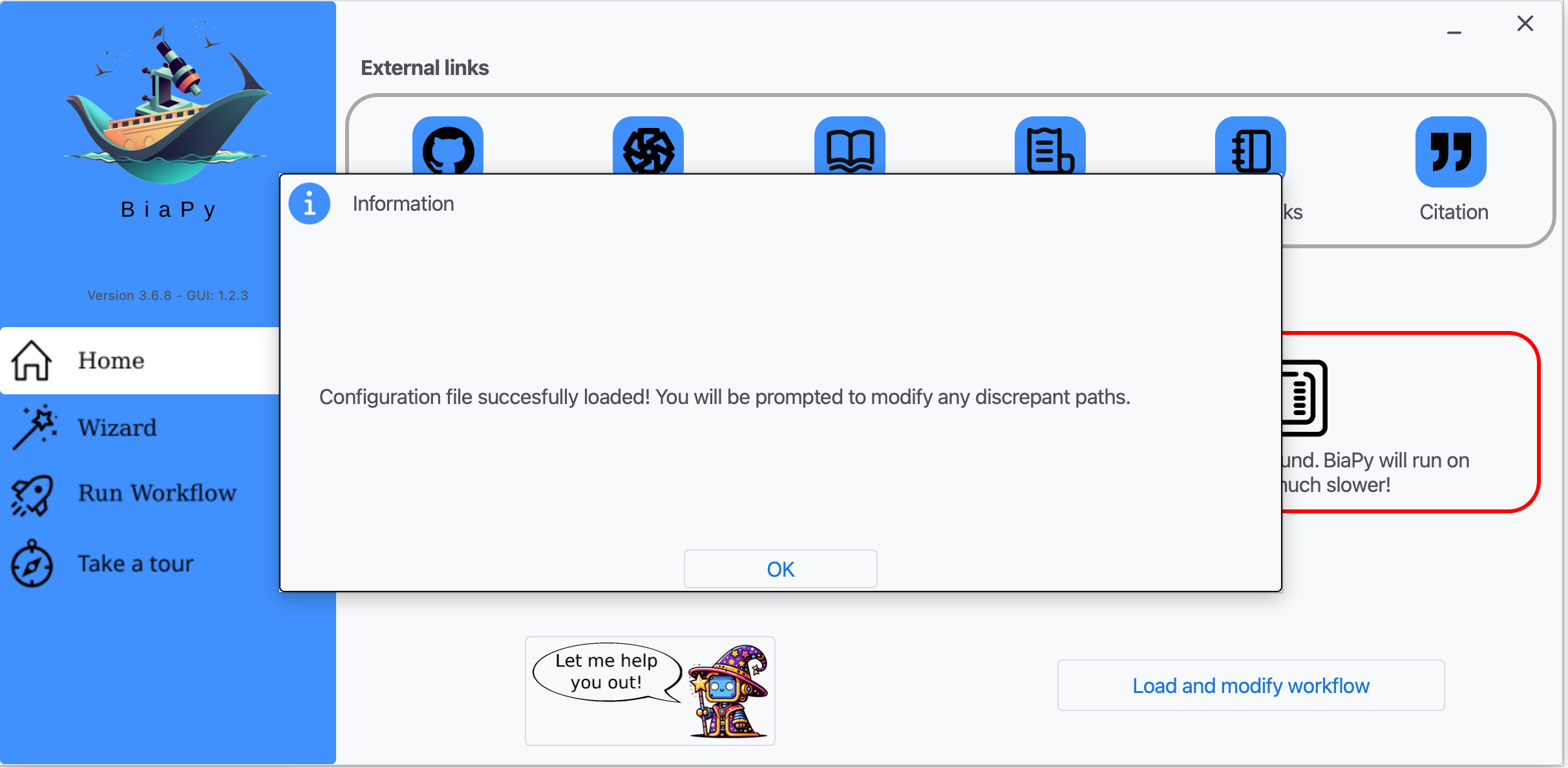
Step 2: Click on "OK".

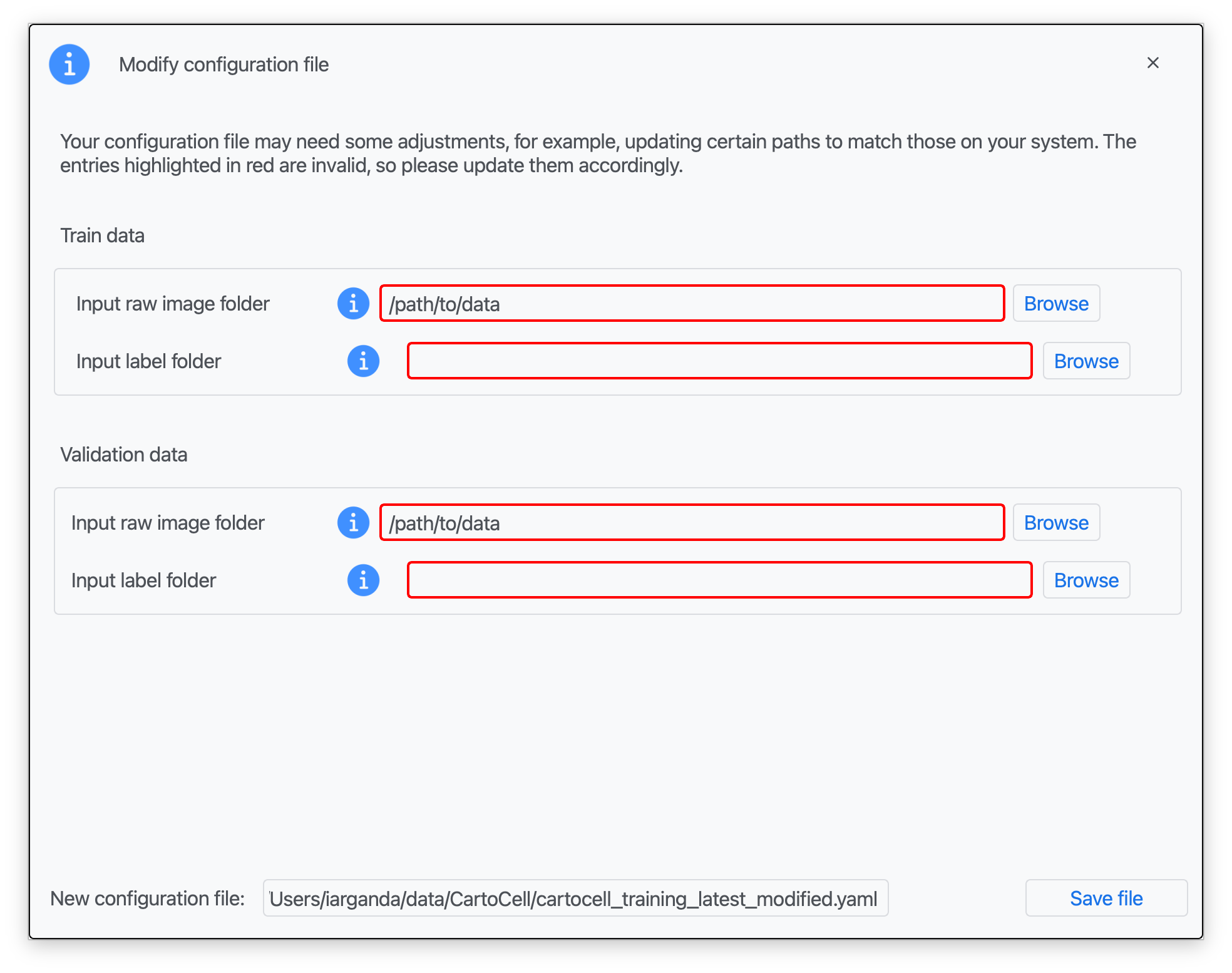
Step 3: Introduce the corresponding paths to your training and validation data (for both raw and label images) and a name for your modified configuration file. Click on "Save file".

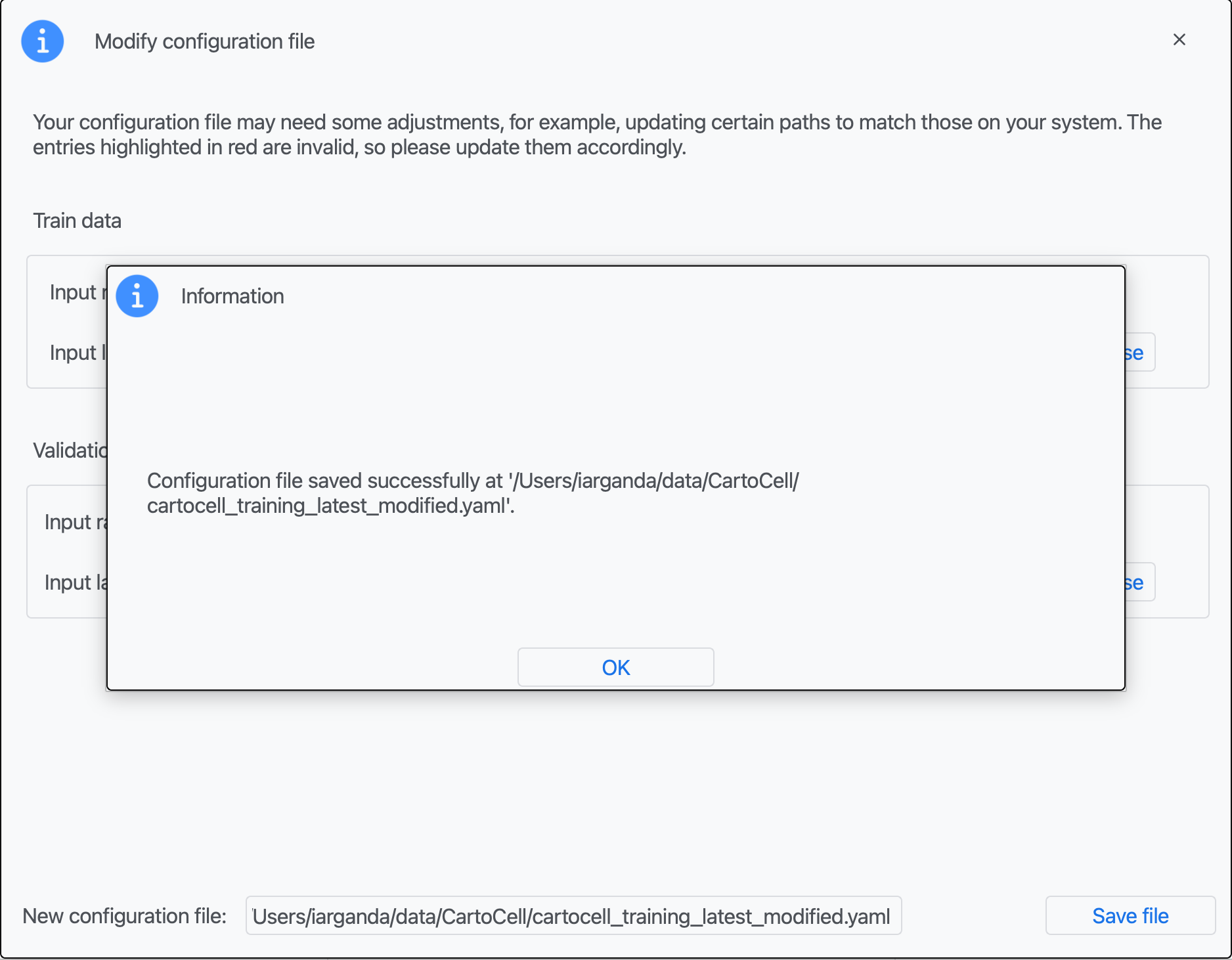
Step 4: You should see an information window indicating the file has been created. Click on "OK".

Step 5: Input the folder you wish to use to store the results of the workflow by clicking on the "Browse" button of "Output folder to save the results" and type a name for your experiment in the "Job name" field.

Step 6: Finally, click on "Check file" and, if a message is displayed showing no errors in the configuration file, click on "Run Workflow".

Previous Next

Note

BiaPy’s GUI requires that all data and configuration files reside on the same machine where the GUI is being executed.

Tip

If you need additional help with the parameters of the GUI, watch BiaPy’s GUI walkthrough video.

Model testing

Again, BiaPy offers different options to run the CartoCell testing (also called inference) workflow depending on your level of computer expertise. Select the one that is most appropriate for you:

GUIGoogle ColabDockerCommand line

First, download CartoCell’s inference configuration file (cartocell_inference_latest.yaml) and our M2 pretrained model (cartocell_M2-checkpoint-best.pth).

Next, in BiaPy’s GUI, follow the following instructions:

Step 1: Click on "Load and modify workflow" and select the 'cartocell_inference_latest.yaml' file you just downloaded.

Step 2: Click on "OK".

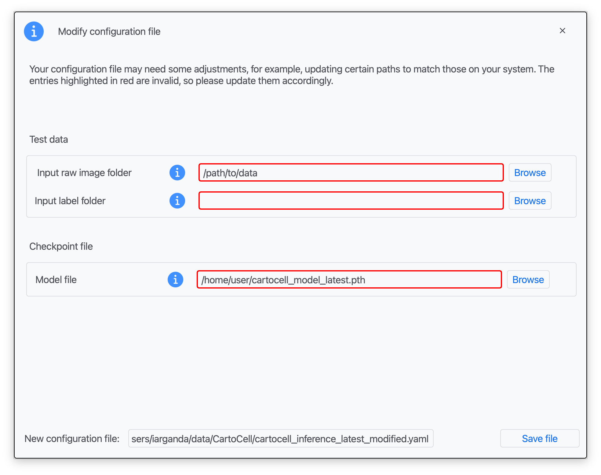
Step 3: Introduce the corresponding paths to your test data (for both raw and label images), the 'cartocell_M2-checkpoint-best.pth' in the "Model file" field and a name for your modified configuration file. Click on "Save file".

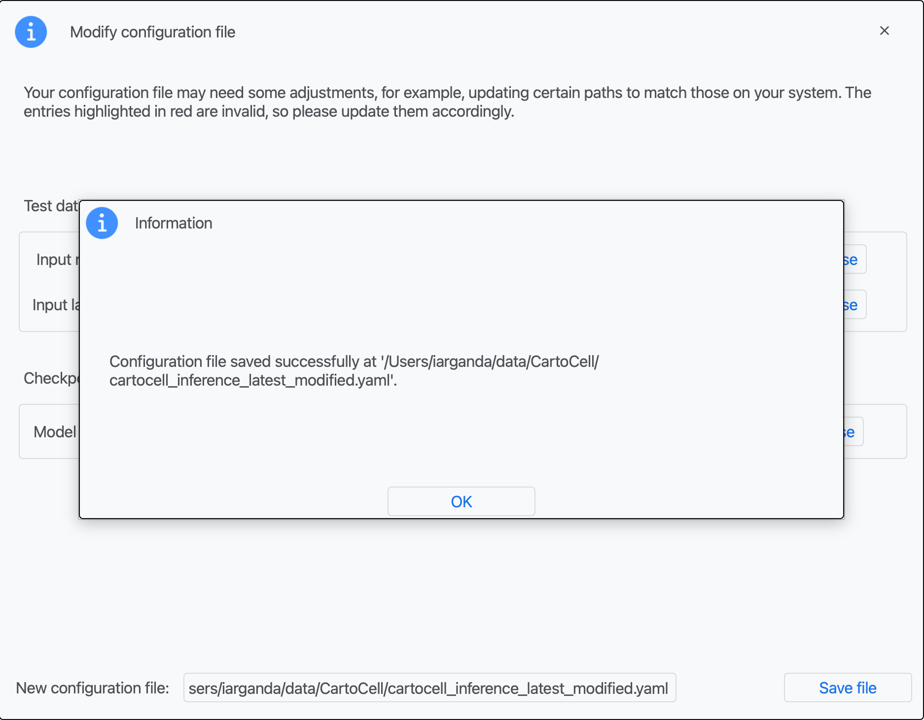
Step 4: You should see an information window indicating the file has been created. Click on "OK".

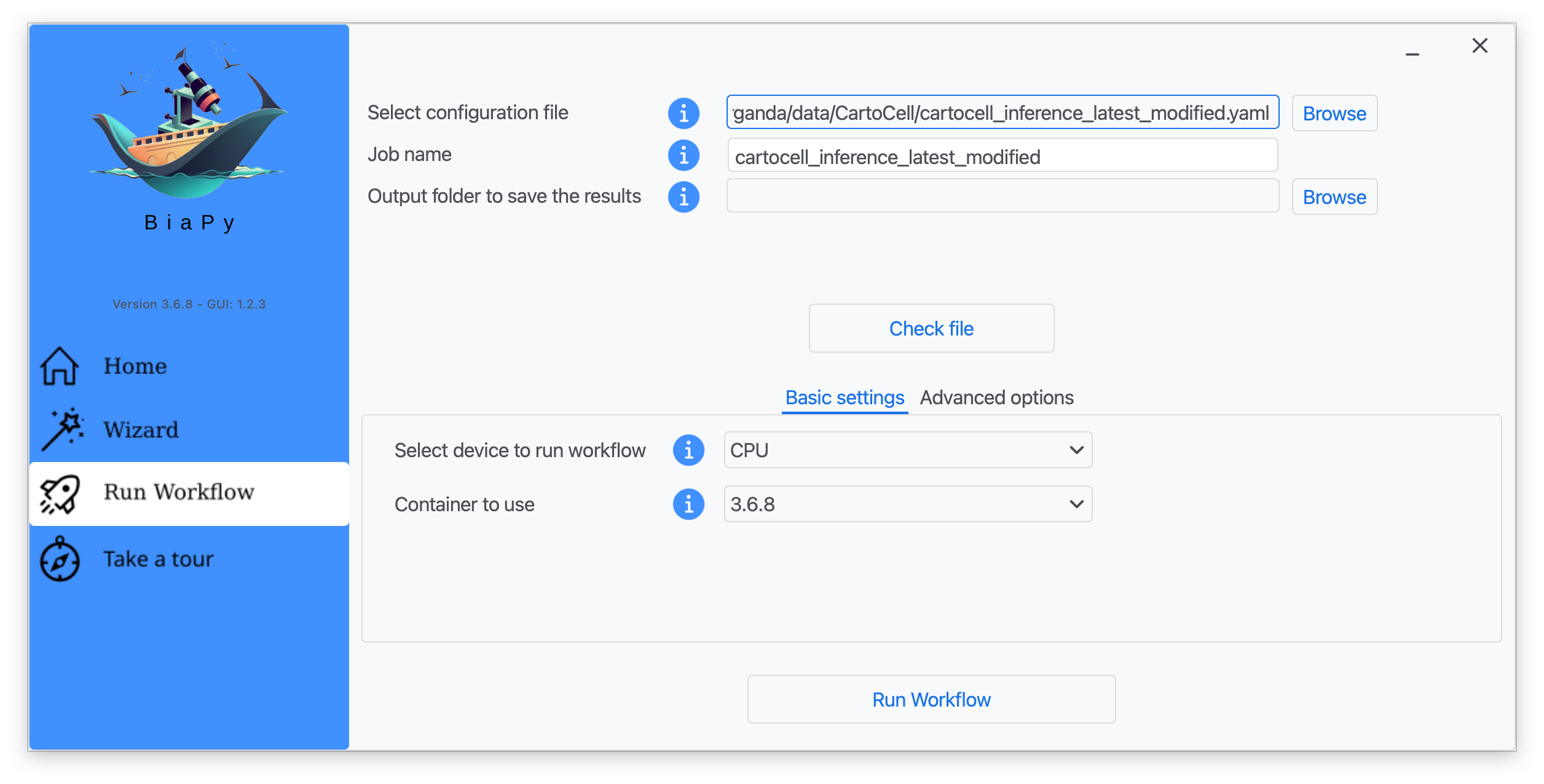
Step 5: Input the folder you wish to use to store the results of the workflow by clicking on the "Browse" button of "Output folder to save the results" and type a name for your experiment in the "Job name" field.

Step 6: Finally, click on "Check file" and, if a message is displayed showing no errors in the configuration file, click on "Run Workflow".

Previous Next

Note

BiaPy’s GUI requires that all data and configuration files reside on the same machine where the GUI is being executed.

Tip

If you need additional help with the parameters of the GUI, watch BiaPy’s GUI walkthrough video.

Results

Training results. Assuming you named your training job cartocell_training, the results of the execution of the workflow should be stored in the folder you defined as result directory, containing a directory tree similar to this:

cartocell_training/
├── config_files/
│   └── cartocell_training_latest.yaml
├── checkpoints
│   └── cartocell_training_latest_1-checkpoint-best.pth
├── train_logs
│   └── cartocell_training_latest_1_log_....txt
└── results
    └── cartocell_training_1
        ├── aug
        │   └── .tif files
        ├── charts
        │   ├── cartocell_training_latest_1_IoU (B channel).png
        │   ├── cartocell_training_latest_1_IoU (C channel).png
        │   ├── cartocell_training_latest_1_IoU (M channel).png
        │   └── cartocell_training_latest_1_loss.png
        └── tensorboard
            └── event.out.tfevents files

Where:

• config_files: directory where the .yaml files used in the experiment is stored.

  • cartocell_training_latest.yaml: the YAML configuration file used for training.

• checkpoints: directory where model’s weights are stored.

  • cartocell_training_latest_1-checkpoint-best.pth: model’s weights file.

• train_logs: directory where training logs are stored.

  • cartocell_training_latest_1_log_2024_12_10_14_01_35.txt: text file with the training log information (the last part of the file name is just an example, since it depends on the time of execution).

• results: directory where all the generated checks and results will be stored. There, one folder per each run are going to be placed.

  • cartocell_training_latest_1: run 1 experiment folder.

    • aug: image augmentation samples.

    • charts:

      • cartocell_training_latest_1_IoU (B channel).png: IoU (Jaccard_index) over epochs plot for the B channel (binary masks).

      • cartocell_training_latest_1_IoU (C channel).png: IoU (Jaccard_index) over epochs plot for the C channel (contours).

      • cartocell_training_latest_1_IoU (M channel).png: IoU (Jaccard_index) over epochs plot for the M channel (foreground mask).

    • tensorboard: TensorBoard visualization related files.

Testing results. Assuming you named your testing job cartocell_inference, the results of the execution of the workflow should be stored in the folder you defined as result directory, containing a directory tree similar to this:

cartocell_inference/
├── config_files/
│   └── cartocell_inference_latest.yaml
└── results
    └── cartocell_inference_1
        ├── per_image
        │   └── .tif files
        ├── per_image_instances
        │   └── .tif files
        ├── per_image_post_processing
        │   └── .tif files
        └── instance_associations
            ├── .tif files
            └── .csv files

Where:

• config_files: directory where the .yaml files used in the experiment is stored.

  • cartocell_inference_latest.yaml: the YAML configuration file used for inference.

• results: directory where all the generated checks and results will be stored. There, one folder per each run are going to be placed.

  • cartocell_inference_1: folder corresponding to the results of the experiment 1.

    • per_image:

      • .tif files: predicted channel images reconstructed from patches.

    • per_image_instances:

      • .tif files: result instance images after watershed.

    • per_image_post_processing:

      • .tif files: same as per_image_instances but applied Voronoi, which has been the unique post-processing applied here.

    • instance-associations:

      • .csv files: six files per test sample summarizing the matches and associations between the predicted instances and the ground truth (if available) with at IoU of 0.3, 0.5 and 0.75.

      • .tif files: one image per test sample showing in colors the different types of matches between the predicted instances and the ground truth (if available) with an IoU of 0.3.

Pre-trained models in the BioImage Model Zoo

Six model M2 variants produced during the CartoCell pipeline are publicly available in the BioImage Model Zoo (BMZ) — a community-driven repository of ready-to-use deep learning models for bioimage analysis. You can find them by searching for “CartoCell” on the BMZ website.

The six CartoCell M2 models available in the BioImage Model Zoo.

These models were evaluated on the CartoCell test set (60 images). The table below ranks them by their mean performance across key segmentation metrics. Three pixel-level IoU (Intersection over Union) scores measure how well the predicted channel images match the ground truth — higher values are better. The instance-level metrics are computed at two IoU matching thresholds — 0.5 (standard) and 0.75 (strict) — and include:

• F1: harmonic mean of detection precision and recall (higher is better).

• PQ (Panoptic Quality): a single score that combines how accurately cells are detected and how well their shapes are segmented (higher is better).

• MTS (Mean True Score): average IoU of correctly matched cell instances (higher is better).

Mean performance of the six CartoCell M2 models on the test set (60 images), sorted by F1 @ IoU threshold 0.5.

Rank	Model	IoU (fg)	IoU (contour)	IoU (mask)	F1 @0.5	PQ @0.5	MTS @0.5	F1 @0.75	PQ @0.75
1	happy-honeybee	0.867	0.542	0.915	0.985	0.814	0.819	0.904	0.758
2	venomous-swan	0.835	0.475	0.878	0.937	0.747	0.773	0.765	0.629
3	idealistic-turtle	0.861	0.494	0.891	0.914	0.731	0.766	0.748	0.616
4	heroic-otter	0.806	0.474	0.858	0.895	0.713	0.748	0.732	0.604
5	intelligent-lion	0.849	0.483	0.874	0.861	0.687	0.752	0.717	0.589
6	merry-water-buffalo	0.837	0.422	0.864	0.578	0.423	0.579	0.279	0.222

Note

happy-honeybee consistently outperforms all other models across every metric, making it the recommended choice for processing new data. merry-water-buffalo achieves competitive pixel-level IoU scores but considerably lower instance-level metrics, suggesting it may struggle to correctly separate individual cells.

All models can be downloaded and run directly through BiaPy or any other BMZ-compatible tool. Visit the BioImage Model Zoo to explore and use them.

Citation

Please note that CartoCell is based on a publication. If you use it successfully for your research please be so kind to cite our work:

Andres-San Roman, J.A., Gordillo-Vazquez, C., Franco-Barranco, D., Morato, L.,
Fernandez-Espartero, C.H., Baonza, G., Tagua, A., Vicente-Munuera, P., Palacios, A.M.,
Gavilán, M.P., Martín-Belmonte, F., Annese, V., Gómez-Gálvez, P., Arganda-Carreras, I.,
Escudero, L.M. 2023. CartoCell, a high-content pipeline for 3D image analysis, unveils
cell morphology patterns in epithelia. Cell Reports Methods, 3(10).
https://doi.org/10.1016/j.crmeth.2023.100597.