Ovarian Reserve: 3D Instance Segmentation of Oocytes

About this tutorial

This tutorial explains how to use BiaPy for 3D instance segmentation of oocytes in whole-mount mouse ovaries, based on “3D Mapping of Intact Ovaries Reveals the Aging Dynamics of the Ovarian Reserve” (bioRxiv, 2025) [2].

The goal is to make this workflow accessible to all BiaPy users (GUI, notebook, Galaxy, Docker, CLI, or API), even if this is your first time working with 3D instance segmentation.

If you still need to install BiaPy, follow the installation guide and choose your preferred option (GUI, Docker, CLI, notebook, etc.) before continuing with the workflow below.

Left: raw DDX4 image stack. Right: corresponding instance-label stack.

Note

A pretrained model is now available for download. You can download it from this SharePoint link. This allows you to directly apply the model to your own ovary images without training from scratch. Alternatively, you can train your own model using the provided training dataset and YAML file (see below).

Paper overview

Our publication [2] presents a pipeline to map the entire ovarian reserve in 3D by imaging intact mouse ovaries with light-sheet fluorescence microscopy (SPIM) and segmenting every individual oocyte with a deep learning model. The key steps of the pipeline are:

1. Whole-ovary SPIM imaging: intact ovaries are cleared and imaged at single-cell resolution across the full organ, yielding large 3D fluorescence volumes (DDX4 channel marking oocyte cytoplasm).

2. 3D instance segmentation with BiaPy: a 3D residual U-Net (ResU-Net) is trained on manually curated oocyte labels using the F + C + Dc channel representation (Binary mask + Contour + Distance to the center), followed by marker-controlled watershed to recover individual instances.

3. Age-resolved quantification: segmented oocyte counts and spatial distributions are compared across seven age groups (5–60 weeks), revealing the dynamics of ovarian reserve decline.

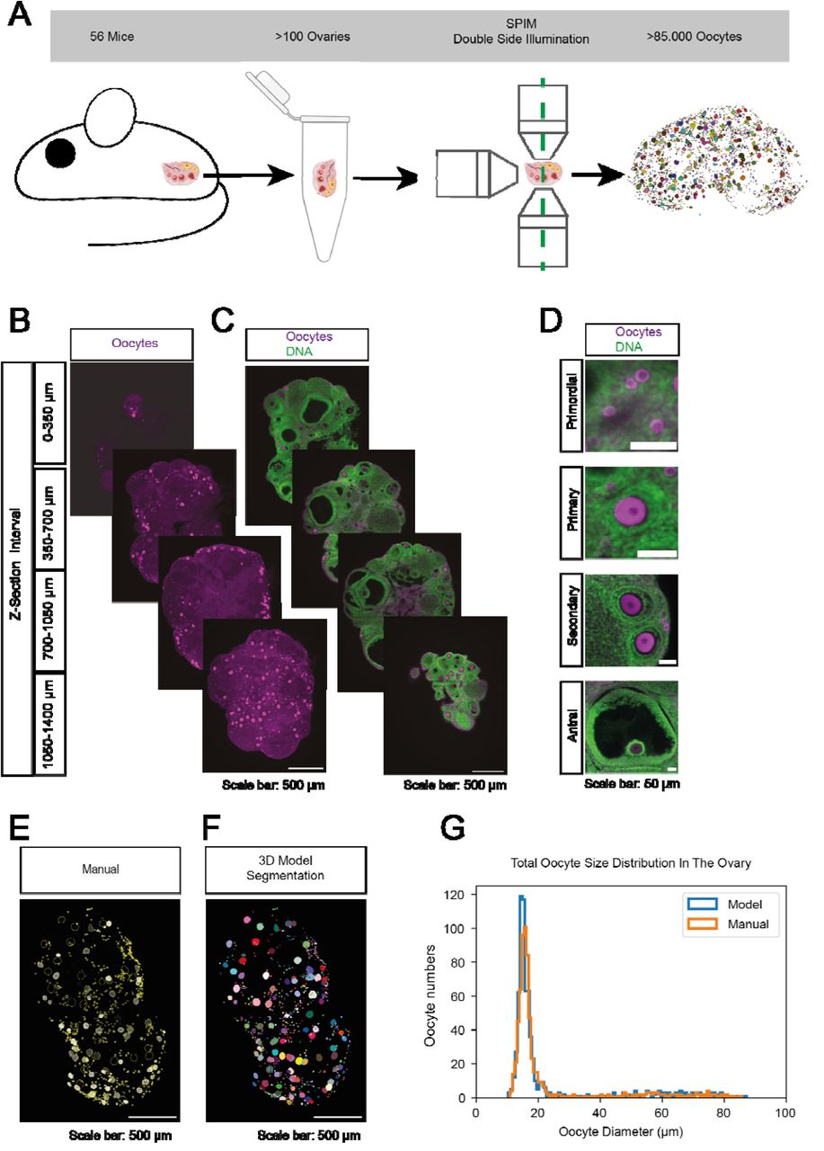
Paper Figure 1 from [2]: SPIM whole-ovary imaging and model-based oocyte segmentation workflow.

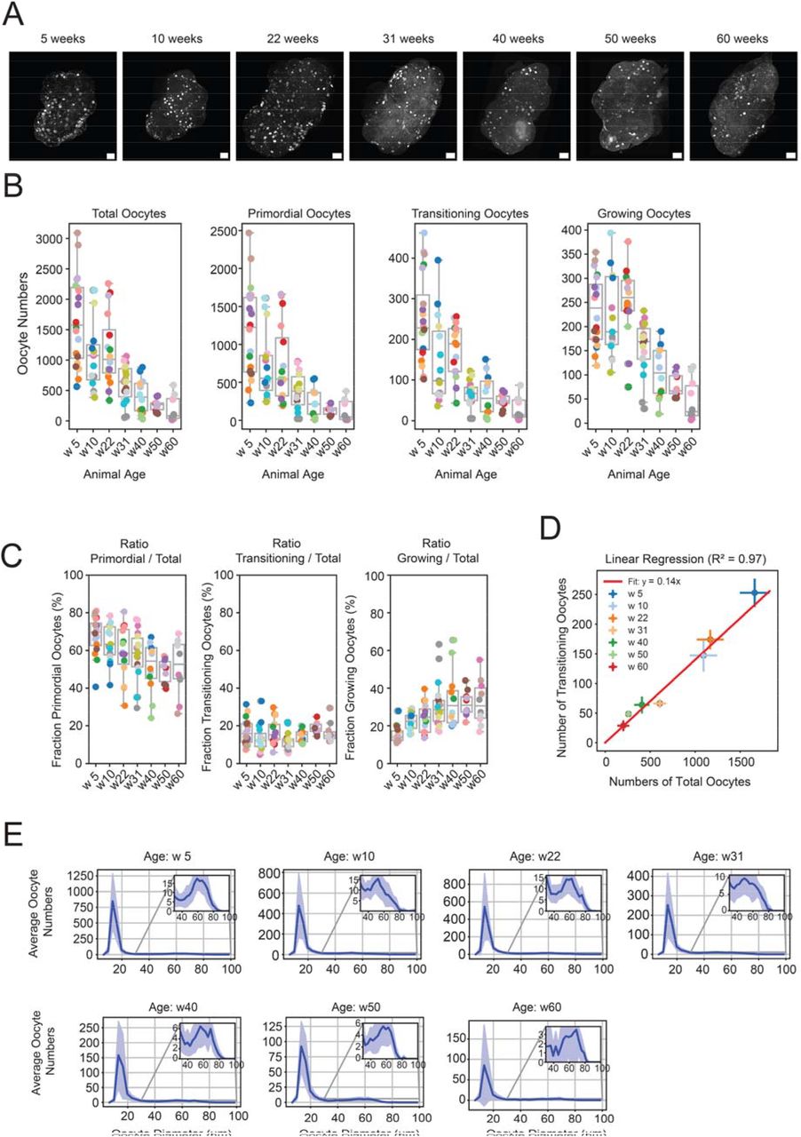
Paper Figure 2 from [2]: age-resolved ovarian reserve quantification enabled by 3D oocyte segmentation.

Data preparation

This tutorial uses two datasets. Note that they represent a small but representative subset of the full data described in [2] — the complete study involved many more labeled slices and full-ovary volumes. These subsets have been selected so that both training and inference (applying the model to new images to produce segmentations) can be completed in a reasonable amount of time on a standard GPU workstation.

The datasets are presented in the natural order of the workflow: first the training data (used to learn the model), then the test data (used to evaluate it).

• Training dataset (sample): oocyte_training.zip (240.9 MB) containing a curated set of paired 3D raw and label image volumes split into training and validation subsets, sufficient to train or fine-tune the segmentation model: OneDrive link.

  Once unzipped, you should find the following directory tree:

  oocyte_training/
  ├── train/
  │   ├── raw/
  │   │   ├── 10W_100330_frame70.tif
  │   │   ├── 10W_105114_1.tif
  │   │   ├── ...
  │   │   └── 5W_150806_frame54.tif
  │   └── label/
  │       ├── 10W_100330_frame70.tif
  │       ├── 10W_105114_1.tif
  │       ├── ...
  │       └── 5W_150806_frame54.tif
  └── val/
      ├── raw/
      │   ├── 10W_100330_fram195.tif
      │   ├── ...
      │   └── 5W_130858_frame89.tif
      └── label/
          ├── 10W_100330_fram195.tif
          ├── ...
          └── 5W_130858_frame89.tif
  

• Test dataset (Zenodo): raw_ovary.rar (13.0 GB) containing seven full 3D ovary volumes covering a range of ages (5, 10, 22, 31, 40, 50, and 60 weeks) in TIFF format. These are a subset of the ovaries analyzed in the paper and serve as the held-out test set: Zenodo link.

  Once unrared, you should find the following directory tree:

  raw_ovary/
  ├── w5_134934.tif
  ├── w10_112648.tif
  ├── w22_090202.tif
  ├── w31_084030.tif
  ├── w40_094116.tif
  ├── w50_142422.tif
  └── w60_155112.tif
  

Image and data requirements

When adapting this pipeline to your own data, the following requirements should be met:

• Input images must be 3D TIFF volumes.

• Typical axis order is ZYX (single channel).

• Expected physical resolution is approximately (5.0, 0.867, 0.867) µm in (Z, Y, X).

• If your data use a different resolution, resampling to this scale is recommended for best results.

Model training

Again, BiaPy offers different options to run this training workflow depending on your level of computer expertise. Select the one that is most appropriate for you:

This training setup uses the OneDrive sample dataset (oocyte_training.zip) as training data and the Zenodo ovary volumes (raw_ovary.rar) as the test set (see Data preparation).

Download the training YAML file here:

• ovarian_reserve_training.yaml

Expand to preview ovarian_reserve_training.yaml

# Ovarian reserve training workflow compatible with recent BiaPy versions

# Problem definition
PROBLEM:
  TYPE: INSTANCE_SEG  # Instance segmentation workflow
  NDIM: 3D            # The model is configured for 3D data
  INSTANCE_SEG:
    DATA_CHANNELS: ["F", "C", "Dc"]    # Prediction targets: Binary mask + Contour + Distance map (to the center)
    DATA_MW_TH_TYPE: auto              # Use automatic watershed thresholds
    DATA_REMOVE_SMALL_OBJ_BEFORE: 10   # Remove tiny objects before watershed (in voxels)
    DATA_REMOVE_BEFORE_MW: true        # Clean predictions before watershed post-processing

# Data paths and preprocessing
DATA:
  NORMALIZATION:
    TYPE: zero_mean_unit_variance      # Standard mean/std normalisation for fluorescence images
    PERC_CLIP:
      ENABLE: True                     # Enable percentile clipping to reduce the influence of outliers during normalization
      LOWER_PERC: 0.1                  # Lower percentile for clipping (e.g., 0.1 means the 0.1th percentile)     
      UPPER_PERC: 99.8                 # Upper percentile for clipping (e.g., 99.8 means the 99.8th percentile)
  PATCH_SIZE: (40, 128, 128, 1)        # Model input patch size: (z, y, x, channels)
  REFLECT_TO_COMPLETE_SHAPE: true      # Mirror-pad borders when shapes are not exact multiples of patch size
  CHECK_GENERATORS: false              # Disable generator preview checks to simplify execution
  TRAIN:
    PATH: "/home/user/oocyte_training/train/raw/"      # Folder with raw training TIFFs (example from oocyte_training.zip)
    GT_PATH: "/home/user/oocyte_training/train/label/" # Folder with matching label TIFFs (example from oocyte_training.zip)
    IN_MEMORY: true                               # Load training data into RAM for faster training if memory allows
  VAL:
    FROM_TRAIN: false  # Use a separate validation set instead of splitting the training data
    PATH: "/home/user/oocyte_training/val/raw/"      # Folder with raw validation TIFFs (example from oocyte_training.zip)
    GT_PATH: "/home/user/oocyte_training/val/label/" # Folder with matching label TIFFs (example from oocyte_training.zip)

# Data augmentation
AUGMENTOR:
  DA_PROB: 0.5          # Probability of applying each augmentation transform
  ENABLE: true          # Enable data augmentation during training
  RANDOM_ROT: true      # Apply random rotations
  VFLIP: true           # Vertical flips
  HFLIP: true           # Horizontal flips
  ZFLIP: true           # Flips along the z axis
  AFFINE_MODE: reflect  # Use reflected borders during geometric transformations
  GRIDMASK: true        # Randomly mask grid-like regions to improve robustness
  GRID_RATIO: 0.7       # Relative size of masked regions in gridmask
  ELASTIC: true         # Elastic deformations to improve invariance to morphology changes

# Deep learning model configuration
MODEL:
  ARCHITECTURE: resunet           # Residual U-Net architecture
  FEATURE_MAPS: [48, 64, 80, 96]  # Number of feature maps at each level of the network
  Z_DOWN: [1, 1, 1]               # Keep z resolution unchanged through downsampling stages
  DROPOUT_VALUES: [0, 0, 0, 0]    # No dropout in this configuration
  LOAD_CHECKPOINT: false          # Start training from scratch; set true to fine-tune from a checkpoint

# Loss function
LOSS:
  CLASS_REBALANCE: True           # Enable class rebalancing to mitigate class imbalance in the instance segmentation representation

# Training configuration
TRAIN:
  ENABLE: true         # Enable training
  OPTIMIZER: ADAMW     # Optimizer used during training
  LR: 1.0e-4           # Initial learning rate
  BATCH_SIZE: 4        # Number of patches per training step
  EPOCHS: 800          # Maximum number of epochs
  PATIENCE: 100        # Early stopping patience
  LR_SCHEDULER:
    NAME: 'warmupcosine'         # Learning rate scheduler with warmup and cosine decay
    MIN_LR: 1.E-5                # Minimum learning rate at the end of cosine decay 
    WARMUP_COSINE_DECAY_EPOCHS: 5 # Number of epochs for the warmup + cosine decay schedule

# Test / inference after training
TEST:
  ENABLE: false       # Disable test/inference in this YAML since it's focused on training; use the separate inference YAML for that workflow

GUIGoogle ColabGalaxyDockerCommand lineAPI

First, download the training configuration file ovarian_reserve_training.yaml.

Next, in BiaPy’s GUI, follow the following instructions:

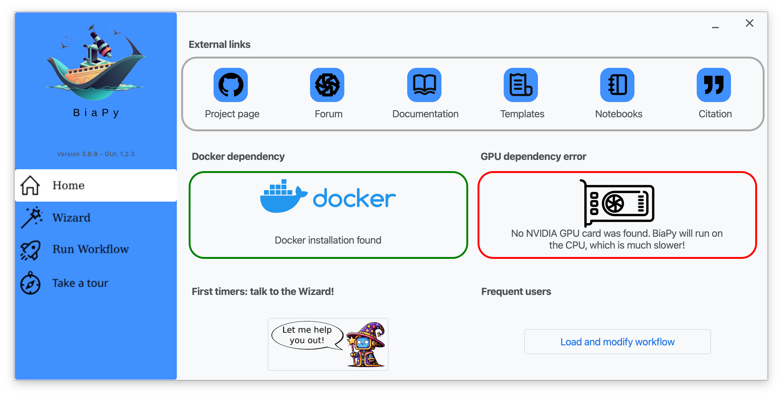
Step 1: Click on "Load and modify workflow" and select the ovarian_reserve_training.yaml file you just downloaded.

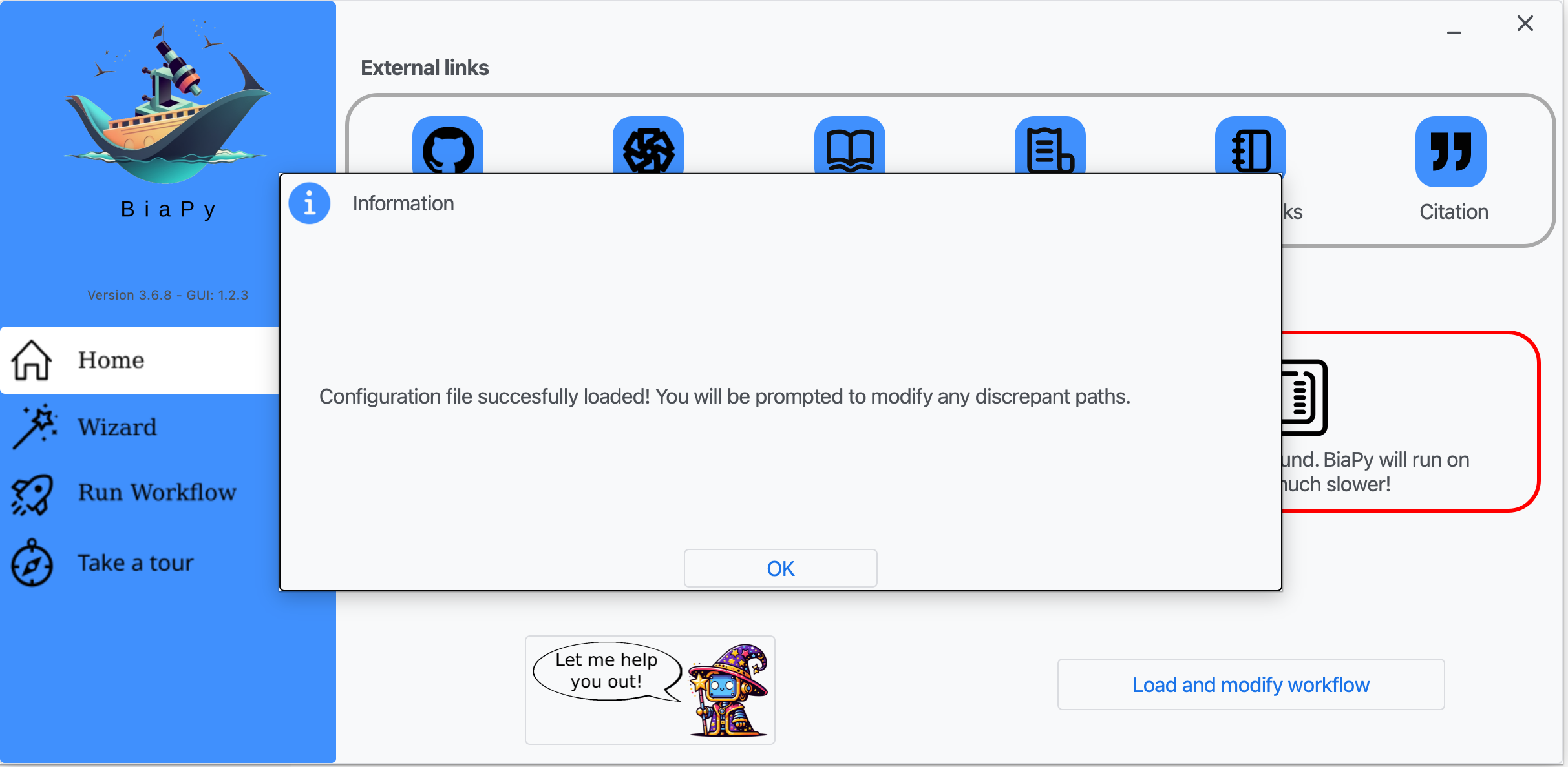
Step 2: Click on "OK".

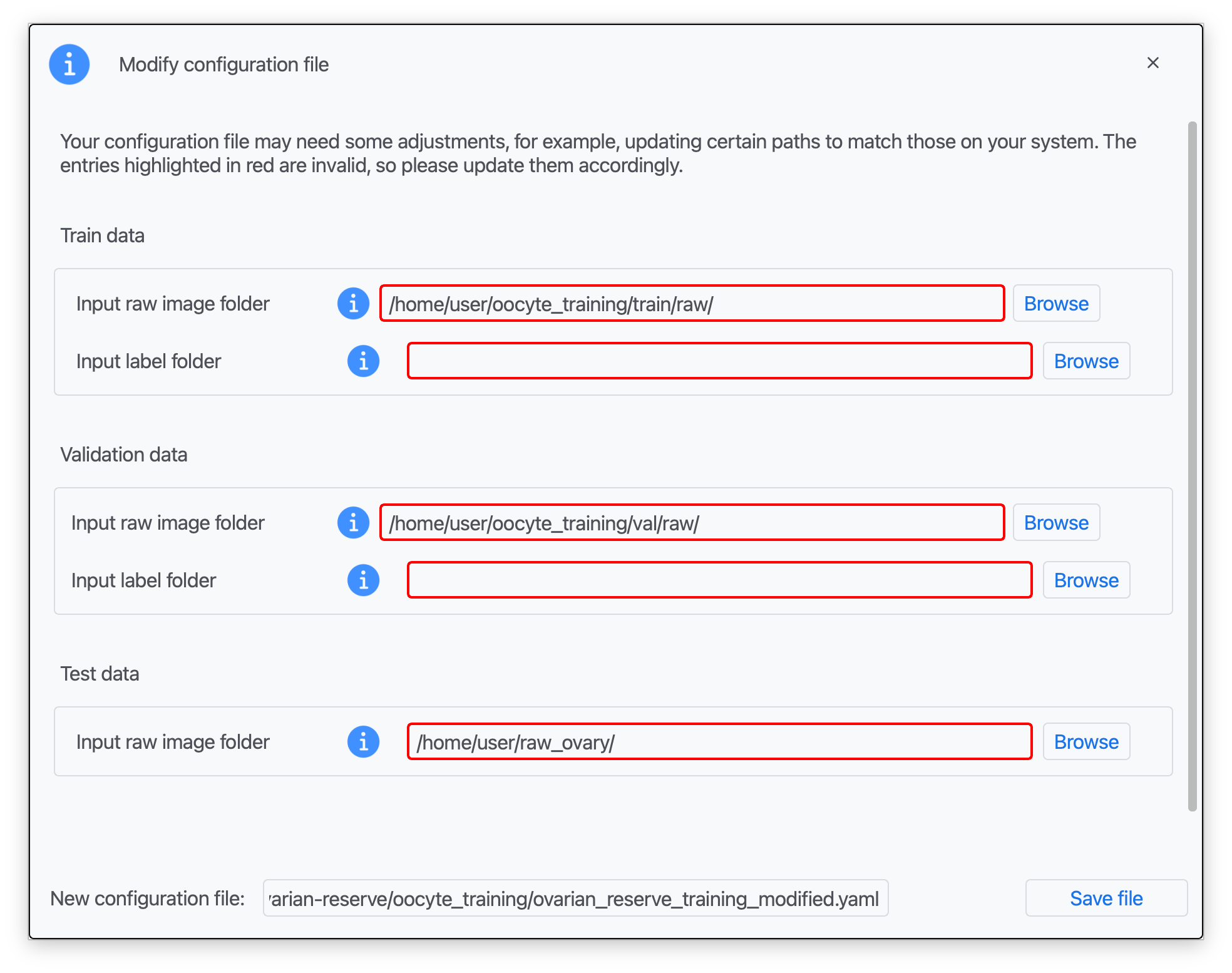
Step 3: Introduce the paths to your training raw and label data (oocyte_training/train/raw/ and oocyte_training/train/label/), validation data (oocyte_training/val/raw/ and oocyte_training/val/label/), set the test path to raw_ovary/ (Zenodo), and type a name for your modified configuration file (see Data preparation; red boxes indicate missing information).

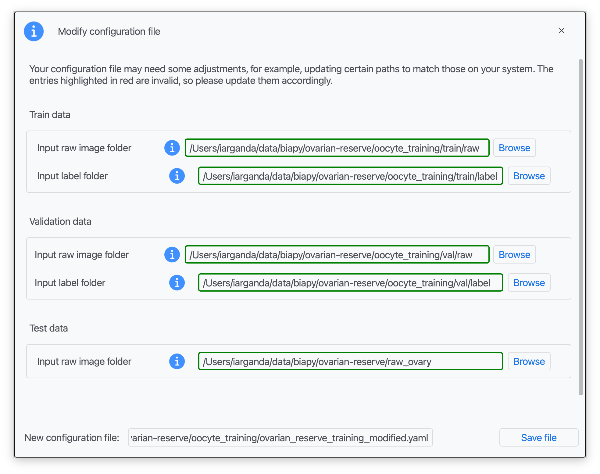
Step 4: Once that information is correctly introduced, click on "Save File".

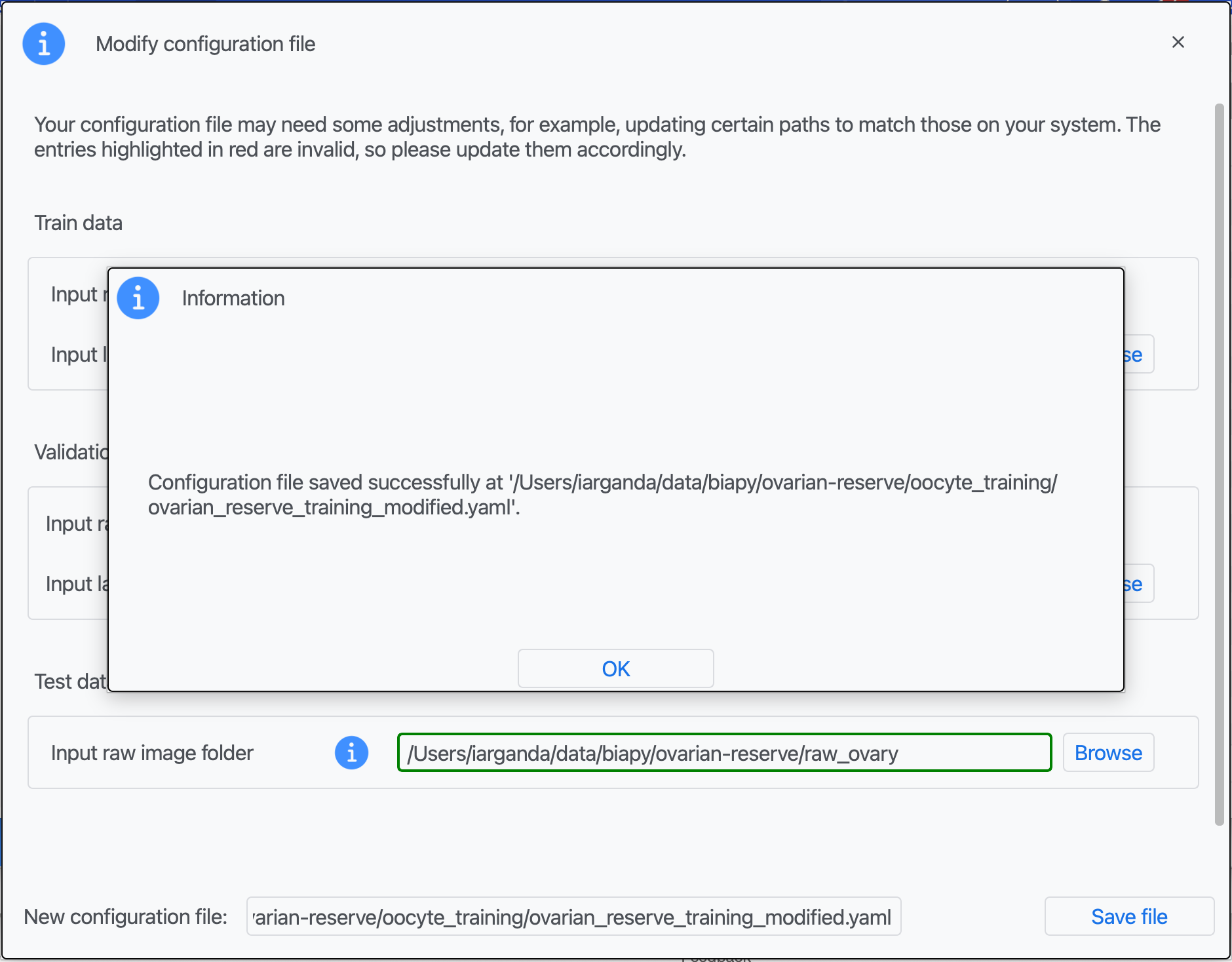
Step 5: A success window should appear. Click on "OK".

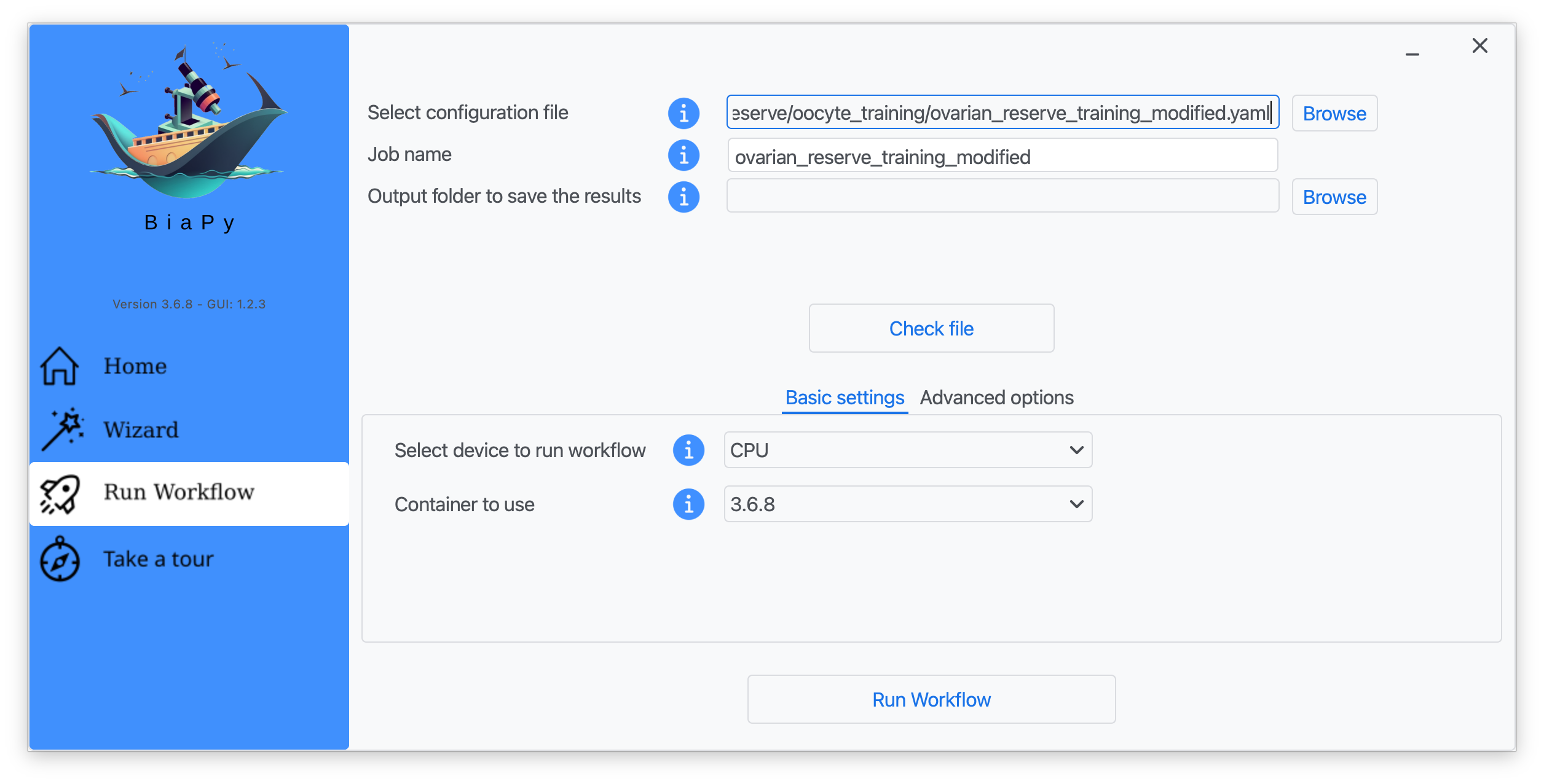
Step 6: Input the folder you wish to use to store the results of the workflow by clicking on the "Browse" button of "Output folder to save the results", and introduce or modify the proposed experiment name in the "Job name" field.

Step 7: Once filled, click on "Check File".

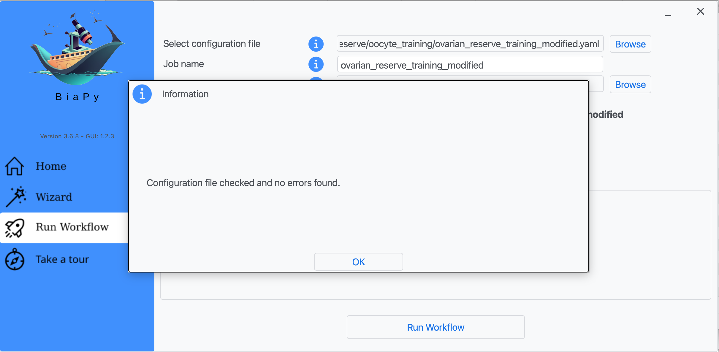
Step 8: A success window should appear. Click on "OK" and then on "Run Workflow".

Previous Next

Note

BiaPy’s GUI requires that all data and configuration files reside on the same machine where the GUI is being executed.

Tip

If you need additional help with the parameters of the GUI, watch BiaPy’s GUI walkthrough video.

Model testing

Again, BiaPy offers different options to run this prediction workflow (also called inference) depending on your level of computer expertise. Select the one that is most appropriate for you:

Download the prediction YAML file here:

• ovarian_reserve_inference.yaml

Expand to preview ovarian_reserve_inference.yaml

# Ovarian reserve inference workflow compatible with recent BiaPy versions

# Problem definition
PROBLEM:
  TYPE: INSTANCE_SEG  # Instance segmentation workflow
  NDIM: 3D            # Input data are 3D volumes
  INSTANCE_SEG:
    DATA_CHANNELS: ["F", "C", "Dc"]    # Prediction targets: Binary mask + Contour + Distance map (to the center)
    DATA_MW_TH_TYPE: auto              # Use automatic watershed thresholds
    DATA_REMOVE_SMALL_OBJ_BEFORE: 10   # Remove tiny objects before watershed (in voxels)
    DATA_REMOVE_BEFORE_MW: true        # Enable object cleanup before marker-controlled watershed

# Data paths and preprocessing
DATA:
  NORMALIZATION:
    TYPE: zero_mean_unit_variance      # Standardise intensities using mean/std normalization
    PERC_CLIP:
      ENABLE: True                     # Enable percentile clipping to reduce the influence of outliers during normalization
      LOWER_PERC: 0.1                  # Lower percentile for clipping (e.g., 0.1 means the 0.1th percentile)     
      UPPER_PERC: 99.8                 # Upper percentile for clipping (e.g., 99.8 means the 99.8th percentile)
  PATCH_SIZE: (40, 128, 128, 1)        # Model input patch size: (z, y, x, channels)
  REFLECT_TO_COMPLETE_SHAPE: true      # Mirror-pad borders if image size is not divisible by patch size
  EXTRACT_RANDOM_PATCH: false          # Do not sample random patches; process the whole test volume by chunks
  TEST:
    PATH: "/home/user/raw_ovary/"            # Folder with Zenodo TIFF volumes or your own TIFF test data
    LOAD_GT: false                            # Ground-truth masks are not required for inference
    IN_MEMORY: false                          # Keep false for large ovaries to reduce RAM usage
    RESOLUTION: (5,0.867,0.867)               # Physical voxel size in microns: (z, y, x)
    OVERLAP: (0,0,0)                          # No overlap between inference patches
    PADDING: (10,32,32)                       # Extra border context added to each chunk during inference

# Deep learning model configuration
MODEL:
  ARCHITECTURE: resunet              # Residual U-Net architecture
  FEATURE_MAPS: [48, 64, 80, 96]     # Number of feature maps at each encoder/decoder level
  Z_DOWN: [1, 1, 1]                  # Do not downsample along z between levels
  DROPOUT_VALUES: [0, 0, 0, 0]       # No dropout in the published configuration
  LOAD_CHECKPOINT: true              # Load pretrained weights from PATHS.CHECKPOINT_FILE

# Path configuration
PATHS:
  CHECKPOINT_FILE: "/home/user/ovarian_reserve_model.pth"  # Full path to the pretrained model checkpoint

# Training section disabled for inference-only workflow
TRAIN:
  ENABLE: false

# Test / inference configuration
TEST:
  ENABLE: true                 # Run inference on test images
  REDUCE_MEMORY: true          # Prefer lower-memory execution for large 3D volumes
  BY_CHUNKS:
    ENABLE: true                           # Process the full ovary volume chunk by chunk
    FORMAT: zarr                           # Internal temporary storage format during chunked inference
    SAVE_OUT_TIF: true                     # Also export final predictions as TIFF files
    INPUT_IMG_AXES_ORDER: ZYX              # Zenodo TIFF volumes are 3D with no explicit channel axis
    WORKFLOW_PROCESS:
      ENABLE: true                        # Reconstruct the full prediction from all chunks
      TYPE: entire_pred                   # Apply the workflow to the entire predicted volume
  POST_PROCESSING:
    MEASURE_PROPERTIES:
      ENABLE: true                        # Measure object properties and optionally remove implausible objects
      REMOVE_BY_PROPERTIES:
        ENABLE: true
        PROPS: [["npixels"], ["sphericity", "npixels"]]  # Properties used to discard artifacts
        VALUES: [[150], [0.01, 2000]]                        # Threshold values for each property rule
        SIGNS: [["le"], ["lt", "lt"]]                    # Comparison operators: <= 150 voxels, sphericity < 0.01, npixels < 2000

Note

If you do not have a checkpoint yet, you can download the pretrained model from this SharePoint link. You can also generate your own checkpoint by following Model training.

Note

The test data are TIFF volumes, and the provided YAML is already configured for TIFF input axis order. Since these volumes are usually large, they are processed internally in chunks as Zarr for efficiency, while final predictions can still be exported as TIFF (controlled with the TEST.BY_CHUNKS.SAVE_OUT_TIF parameter).

GUIGoogle ColabGalaxyDockerCommand lineAPI

First, download the prediction configuration file ovarian_reserve_inference.yaml and prepare a pretrained .pth model checkpoint (either your own from Model training or the provided pretrained model from the SharePoint link above).

Next, in BiaPy’s GUI, follow the following instructions:

Step 1: Click on "Load and modify workflow" and select the ovarian_reserve_inference.yaml file you just downloaded.

Step 2: Click on "OK".

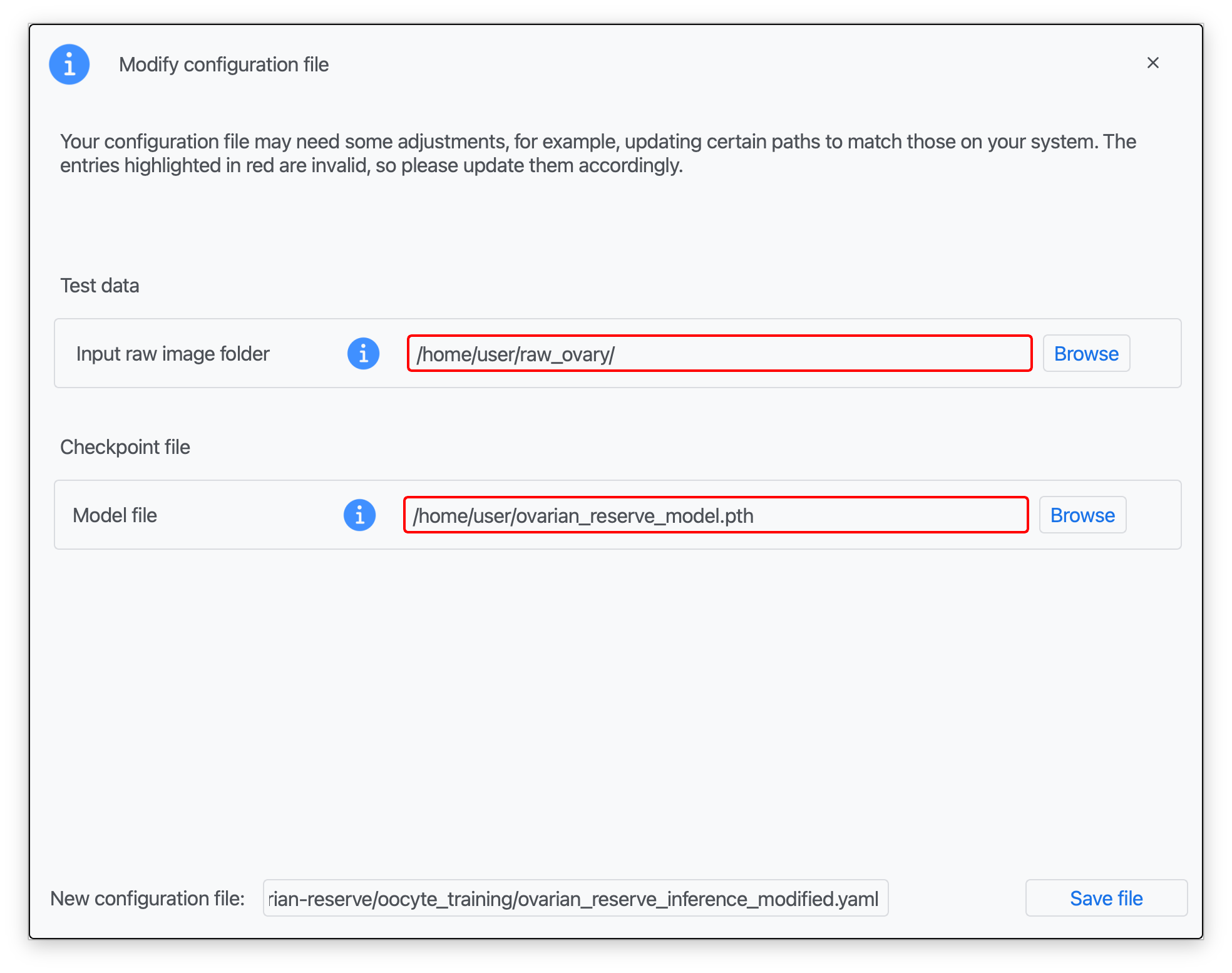
Step 3: Introduce the corresponding paths to your test data (raw images), a pretrained .pth model file, and a name for your modified configuration file (see Data preparation; red boxes indicate missing information).

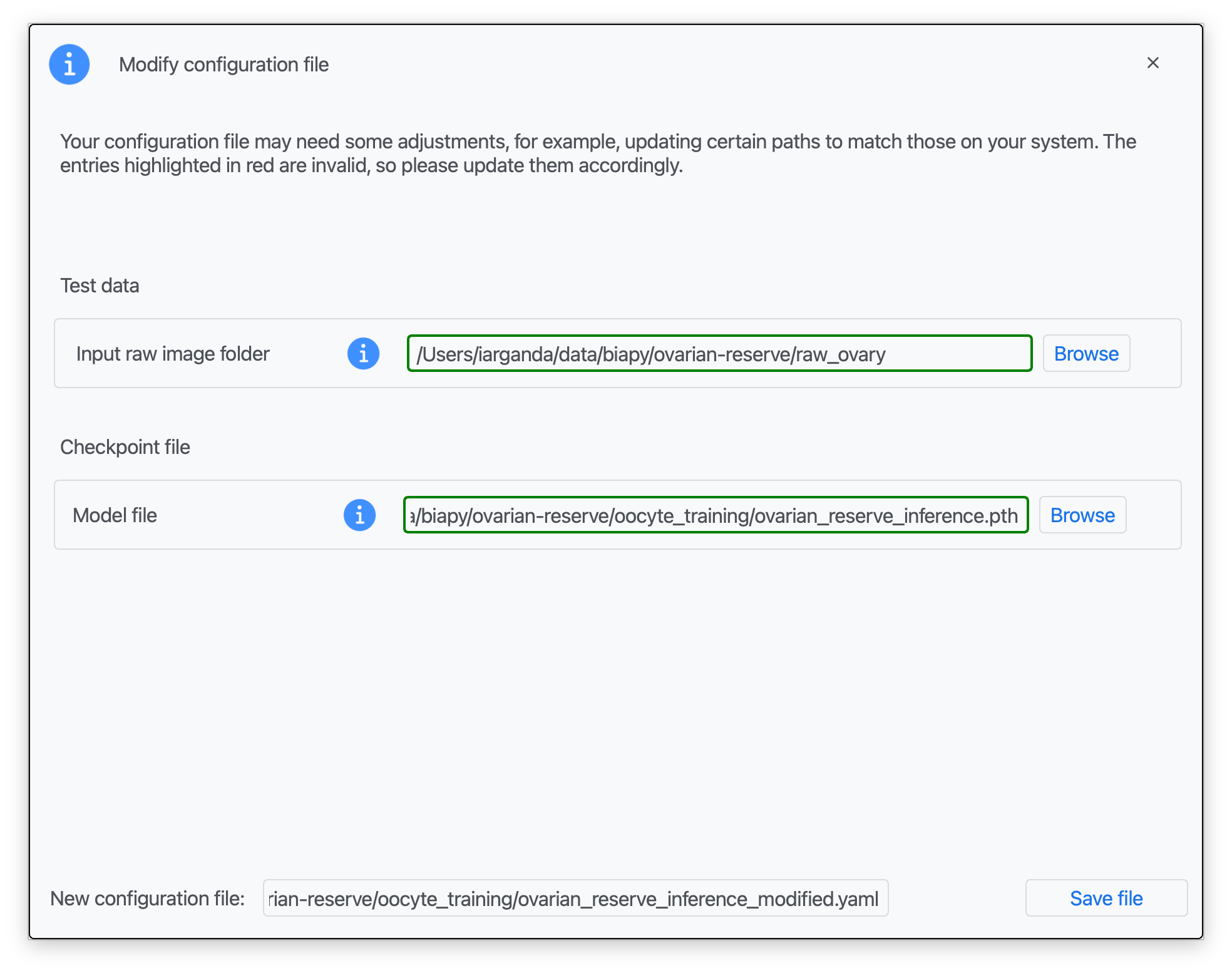
Step 4: Once that information is correctly introduced, click on "Save File".

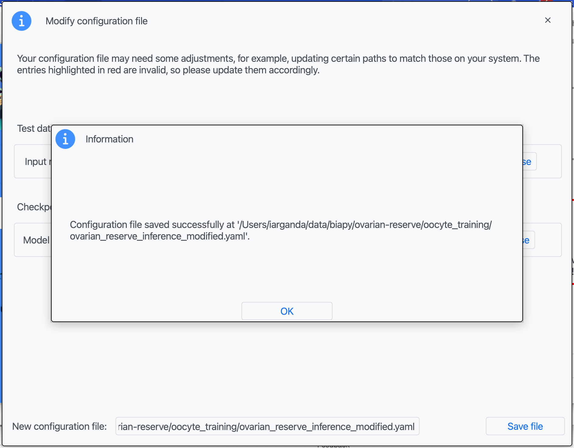
Step 5: A success window should appear. Click on "OK".

Step 6: Input the folder you wish to use to store the results of the workflow by clicking on the "Browse" button of "Output folder to save the results".

Step 7: Once filled, click on "Check File".

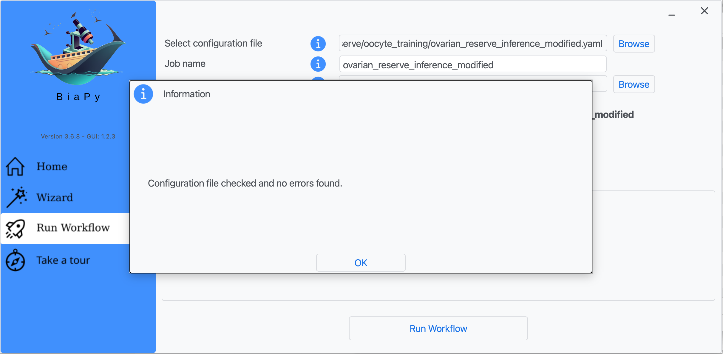
Step 8: A success window should appear. Click on "OK" and then on "Run Workflow".

Previous Next

Note

BiaPy’s GUI requires that all data and configuration files reside on the same machine where the GUI is being executed.

Tip

If you need additional help with the parameters of the GUI, watch BiaPy’s GUI walkthrough video.

Results

Training results. Assuming you named your training job my_ovarian_reserve_training, the results should be stored in the folder defined in result_dir, with a structure similar to this:

my_ovarian_reserve_training/
├── config_files/
│   └── ovarian_reserve_training.yaml
├── checkpoints/
│   └── my_ovarian_reserve_training_1-checkpoint-best.pth
├── train_logs/
│   └── my_ovarian_reserve_training_1_log_....txt
└── results/
    └── my_ovarian_reserve_training_1/
        ├── aug/
        ├── charts/
        └── tensorboard/

Where:

• config_files: directory where YAML files used in the experiment are stored.

• checkpoints: directory where model weights are stored.

• train_logs: directory where training logs are stored.

• results: directory where generated checks and outputs are stored, with one subfolder per run.

Testing results. Assuming you named your testing job my_ovarian_reserve_test, the results should be stored in the folder defined in result_dir, with a structure similar to this:

my_ovarian_reserve_test/
├── config_files/
│   └── ovarian_reserve_inference.yaml
└── results/
    └── my_ovarian_reserve_test_1/
        ├── per_image/
        ├── per_image_instances/
        ├── per_image_post_processing/
        └── instance_associations/

Where:

• config_files: directory where YAML files used in the experiment are stored.

• results: directory where generated checks and outputs are stored, with one subfolder per run.

• per_image: reconstructed output channel predictions.

• per_image_instances: final instance segmentations.

• per_image_post_processing: instance predictions after post-processing.

• instance_associations: optional CSV/TIFF summaries of instance matching against ground truth (if available).

Pre-trained models in the BioImage Model Zoo

The model produced during this study is publicly available in the BioImage Model Zoo (BMZ) — a community-driven repository of ready-to-use deep learning models for bioimage analysis. It’s name is plucky-leopard and can be found in this link: https://bioimage.io/#/artifacts/plucky-leopard.

The oocyte segmentation model (plucky-leopard).

Note

The model can be downloaded and run directly through BiaPy or any other BMZ-compatible tool. Find more information about how to use BMZ models in BiaPy in BioImage Model Zoo documentation section.

Post-analysis scripts

After segmentation, you can run the analysis scripts from the Boke-Lab ovarian_reserve repository:

• oocyte density: quantifies oocytes per volume.

• radial quantification: measures the radial spatial distribution of oocytes.

These scripts reproduce the quantitative analyses described in [2].

Citation

Please note that this tutorial is based on a publication. If you use it successfully for your research, please cite our work:

3D Mapping of Intact Ovaries Reveals the Aging Dynamics of the Ovarian Reserve
Arturo D'Angelo, Daniel Franco-Barranco, Marco Musy, James Sharpe, Ignacio Arganda-Carreras,
Elvan Böke
bioRxiv 2025.11.07.686728; doi: https://doi.org/10.1101/2025.11.07.686728